"The theory of probabilities is just common sense reduced to calculus."

Pierre-Simon Laplace

This document contains an introduction to probibalistic inference meant as a comfortable first step for data people to get introduced to bayesian thinking. It will be a bit mathy, but nothing beyond kahn-level probability.

Definition

Bayes Rule is a lovely law in probability theory that is defined via a simple formula.

$$ P(E|D) = \frac{P(E,D)}{P(D)} = \frac{P(D|E)P(E)}{P(D)} $$

Here $E$ and $D$ are events. They can be anything. As a simplest example; suppose that I am rolling dice and that $D$ is the number of dice that I've rolled and that $E$ is the number of eyes that I see. Via some basic simulation I can generate plots of what $P(E|D)$ might look like.

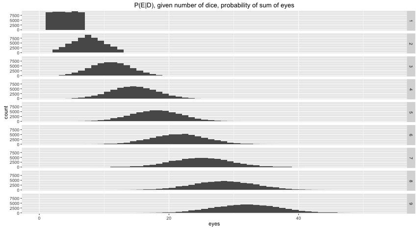
In this plot you see the probability distribution for the number of eyes given the number of dice that are rolled. The number of dice are listed on the right hand side, the number of eyes are denoted on the x-axis and the y-axis shows how often this occured in a simulation. You should notice that when I roll 4 dice that it is not likely for me witness a total of 4 eyes but it is impossible to get 3. This is what we expect and this is what we could also calculate with probability theory.

Here's an amazing thing; you could turn this plot on it's head. If you only switch the numbers on the x-axis with the numbers on the right hand side then you suddenly have all distributions for $P(D|E)$. We can use what we know about $P(E|D)$ to gain knowledge about $P(D|E)$. As we'll see in the next formal example, this is a very nice property and it's something that follows straight from probability theory.

A textbook example

Let's consider a textbook problem, this time with a bit more math;

There is an epidemic. A person has a probability $\frac{1}{100}$ to have the disease. The authorities decide to test the population, but the test is not completely reliable: the test generally gives $\frac{1}{110}$ people a positive result but given that you have the disease the probability of getting a positive result is $\frac{65}{100}$.

Let $D$ denote the event of having the disease, let $T$ denote event of a positive outcome of a test. If we are interested in finding $P(D|T)$ then we can just go and apply Bayes rule:

$$ P(D|T) = \frac{P(T|D)P(D)}{P(T)} = \frac{\frac{65}{100} \times \frac{1}{100}}{\frac{1}{110}} \approx 0.715 $$

This is neat. We learned something about having the disease via our knowledge on the performance of the test. Bayes rule gives us a precise method to generate more knowledge after having observed data. In this case the data that we observe is the fact that the test was positive. What else can we calculate?

More inference $P(T|\neg D)$

Suppose that you do not have the disease, can the test come out positive?

We can use basic probability theory again and split up the probability of getting a positive test result. It's easier to think about this outcome by splitting it up into two situations; the situation that multiple tests are positive given that you have the disease and the situation that multiple tests are positive given that you don't have the disease.

$$ \begin{align} P(T) & = P(T\cap D) + P(T\cap \neg D) \\ & = P(T|D)P(D) + P(T|\neg D)P(\neg D) \end{align} $$

We know $ P(T|D) $ , $P(D)$ and $P(T)$. We can figure out that $P(\neg D) = 1 - P(D)$ too. So we only need to fill these numbers into the formula above to get;

$$P(T|\neg D) = \frac{19}{7260}$$

Taking more tests

Sofar, we've only considered the outcome of one test. Again we can think about what the probability might be that two tests are both positive by splitting the situation up into the two possibilities for getting the disease.

\begin{align} P(TT) &= P(TT|D)P(D) + P(TT| \neg D) P(\neg D) \\ &\approx 0.004237374 \end{align}

\begin{aligned} P(TTT) &= P(TTT|D)P(D) + P(TTT| \neg D) P(\neg D) \\ &\approx 0.002746294 \end{aligned}

Notice that these probabilities were not strictly given to us. These are probabilities that we've inferred from the information known to us by applying probability theory. The only true assumption that we've made is that the only thing that is of influence to the test result is wheather or not you have the disease.

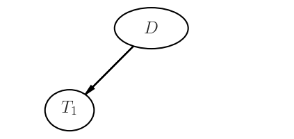
Graphical View

People tend to get lost in the math a bit here, so it might be good to introduce a visual method of communicating.

$$ P(D|T) = \frac{P(T|D)P(D)}{P(T)} = \frac{\frac{65}{100} \times \frac{1}{100}}{\frac{1}{110}} \approx 0.715 $$

Multiple Tests

In the next bit I'll introduce a graphical notation along with the any math. Let's figure out how likely it is to have a certain disease after taking one, two or three tests that came out positive. We'll use results that we've calculated before.

Two Tests

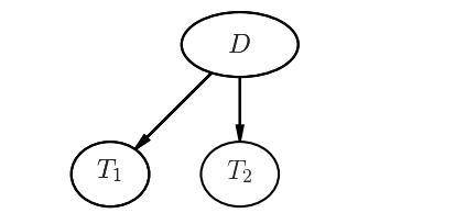
$$ P(D|TT) = \frac{P(TT|D)P(D)}{P(TT)} \approx 0.9971 $$

Three Tests

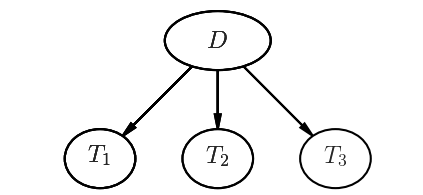
$$ P(D|TTT) = \frac{P(TTT|D)P(D)}{P(TTT)} \approx 0.9999$$

What just happened?

Via Bayes Rule, we can infer information about $P(D|TTT)$ even though we initially only know about $P(T|D)$ (and $P(T)$ and $P(D)$).

The trick is that we clearly define the uncertainty that we have and infer the rest via probability theory. In this case the main cheat was realizing that the tests are independant of eachother. This is what makes inference so strong! By defining our uncertainties in how we model things we can use probability theory to infer knowledge once data is known to us.

Even More Inference!

Let's have another look at this graphical representation.

This graph describes how a system of dependencies which define probabilities of events. Be careful though. This graphical representation should not suggest that the inference can only occur in one direction.

For example, suppose that we took two tests that were both positive, how would our belief change for the third test (ie: what is $P(T_3|T_1, T_2)$)?

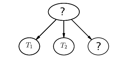
You can describe the sensation of inference through words as well. If two tests are positive, it is very likely that you have the disease. If it is very likely that you have the disease then it is also rather likely that the next test is positive.

In maths;

$$ P(T_3 | T_1 T_2 ) = \frac{P(T_1, T_2, T_3)}{P(T_1, T_2)} = \frac{1076657}{1661220} \approx 0.6481 $$

Note that there's an alternative method (this is a longer path, but worthwhile to understand if you've never walked this road before).

\begin{align} P(D | T_1, T_2) & = \frac{16731}{16780} \\ P(\neg D | T_1, T_2) & = 1 - P(D | T_1, T_2) = \frac{49}{16780} \end{align}

\begin{align} P(T_3 | T_1, T_2) & = P(T_3 | T_1, T_2, D) P(D | T_1, T_2) + P(T_3 | T_1, T_2, \neg D) P(\neg D | T_1, T_2) \\ & = P(T_3 | D) P(D | T_1, T_2) + P(T_3 | \neg D) P( \neg D | T_1, T_2) \\ &\approx 0.6481 \end{align}

Notice that 0.6481 is almost the same as $P(T|D)$, which is what we would expect.

The graphical representation tells us that once we know $D$ the events $T_1 ... T_3$ are independant of eachother. That doesn't mean that we cannot infer about $P(D | T_i)$, it merely means that we have to keep track of different assumptions in our model. Probability theory resolves the rest.

Conclusion

Please recognize how powerful this methodology is. Not only does this way of thinking give you immense modelling flexibilities but it even allows you to work with actual probabilities at all times. Many machine learning models try to approximate this thinking with more black box sort of methods but it loses some probibalistic interpretation in the process.