The k-means algorithm is great, but people tend to always get into discussions on how to choose the parameter $k$. In this blogpost I will demonstrate a simple bayesian method to automate this decision a bit $k$.
The task
We will want to apply k-means on the following 1-dimensional dataset:
library(ggplot2)
library(stringr)
library(dplyr)
library(purrr)
library(tidyr)

n <- 2000
df <- data.frame(x = c(rnorm(n), rnorm(n, 4), rnorm(n/2, -3.5)))

ggplot() +
  geom_density(data=df, aes(x), fill = "steelblue", colour = NA) +
  ggtitle("shape of the data")
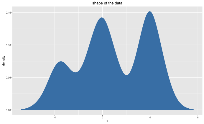
Preferably, we would do a k-means clustering where $k=3$. The algorithm may consider other values of $k$ but it needs to come to the conclusion that this is subobtimal.
Theory
Take $H$ to be a hypothesis (say $k=4$ or $k=8$) and let $D$ be the data that is observed. We are keen on finding $ P(H|D) $ such that we may take the hypothesis with the largest probability given the data. Luckily, we have bayes rule, which has some interesting implications.
$$ P(H|D) = \frac{P(D|H)P(H)}{P(D)} \propto P(D|H)P(H)$$
Let's zoom in on $P(D|H)$. It calculates, for every hypothesis, what the probability is that the data that we have is generated from via a certain hypothesis. This likelihood, we will find out, punishes complicated models without the need of putting our own priors in about the preference of each hypothesis ($P(H)$). For the rest of this document I'll assume $P(H)$ to be homegeneous for all hypotheses.
Note that we are not interested in finding the exact probability value $P(H|D)$; we can suffice with a likelihood than can just tell us which hypothesis is most likely.
Code
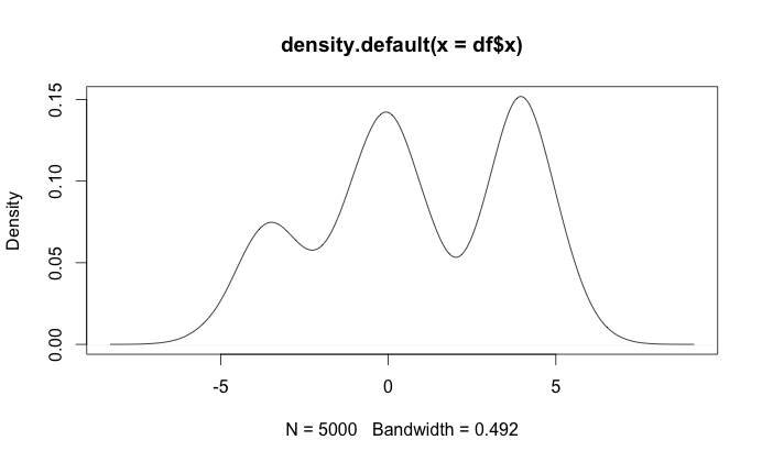
R comes with a very nice density function, which uses gaussian kernels to do a nonparametric estimation of the density. In laymans terms: it can estimate the density for us, which is useful when we want to calculate $P(D|H)$.
dens <- density(df$x)
dens %>% plot
The following code generates likelihoods for different values of $k$ as well as generates a dataframe with the likelihood estimate for every allocation of clusters.
find_density <- function(dens_obj, x){
  index <- (dens_obj$x - x) %>% abs %>% which.min
  dens_obj$y[index]
}

pltr <- data.frame()
lik <- data.frame()

for(i in 1:12){
  # perform kmeans for k=i
  mod <- kmeans(df$x, i)
  sizes <- mod$cluster %>% table %>% array
  centers <- mod$centers

  # sample data from this kmeans allocation
  # such that we can estimate a density
  sampled_data <- map2(sizes, centers, ~ rnorm(.x, .y)) %>% unlist
  dens <- density(sampled_data)

  # calculate likelihood that this density
  # create the data we started out with
  likelihood <- df$x %>%
    map(~find_density(dens, .) %>% log) %>%
    reduce(sum)

  # update dataframes that keep track of data
  pltr <- rbind(pltr, data.frame(x = dens$x, y = dens$y, i = i))
  lik <- rbind(lik, data.frame(k = i, likelihood = likelihood))
}
Note that to determine the sample size for each cluster, I count the number of points that are assigned to it. For every clustering allocation we now have an associated density $p(x|H)$. This is what they look like:
ggplot() +
  geom_line(data=pltr, aes(x,y)) +
  facet_wrap(~i, scales = "free") +
  ggtitle('which likelihood is the most similar')
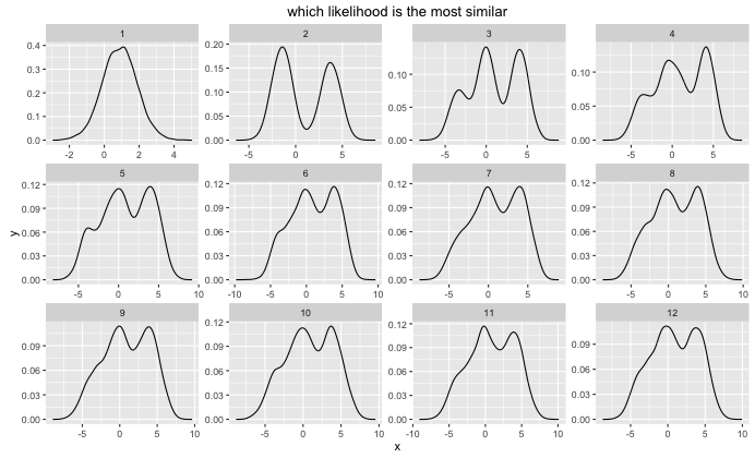
The only trick applied here is that I try to fit my original data with each of these distributions via map(~find_density(dens, .) %>% log) and get a log likelihood. These are summerized in the table below.
> lik
    k likelihood
1   1  -26040.41
2   2  -13183.14
3   3  -11850.67
4   4  -11939.20
5   5  -12039.32
6   6  -12077.95
7   7  -12090.67
8   8  -12104.20
9   9  -12134.48
10 10  -12132.03
11 11  -12148.86
12 12  -12130.69
Behold(!), we reach maximum likelihood when we only have 3 clusters. By simply looking at bayes theorm we have gotten ourselves a probibalistic way of finding an appropriate $k$.
Conclusion
I've kept the example simple by keeping $\sigma = 1$ everywhere. In practice this would be another thing that you estimate, but the general likelihood rule would still apply. In practice the likelihood function would just get (much) more complicated but you would still be able to apply a similar $P(D|H)$ trick to pick the best model.
Note that this trick can be applied for other models and other tasks as well. Bayes rule is suprisingly effective in suggesting clever ways to judge algorithms. The hard part of these types of algorithms usually isn't in the application of bayes theorem, rather in finding an appropriate sampler. Because we're only using a one dimensinal problem we can use the simple density method. For more dimensions I might advice the kernel density estimator from scikit learn, which is quite exellent!