So here's an interesting question;
Can we generate a meaningful regression out of randomness?
You may be tempted to think that this is impossible because randomness does not contain any information. Although this is a valid statement I'd like to show the contrary in this blogpost. Turns out that correlated entropy can generate useful features that can be used to fit smooth functions.
Libraries
I'll demo this approach in R, to follow along you'll need the following libraries installed;
library(dplyr)
library(ggplot2)
library(tidyr)
Biased Entropy Series
Let's generate some random, but correlated, data. The idea is that this data will later generate a sequence.
These two slides from Ian Murray might explain the idea better than words or math.
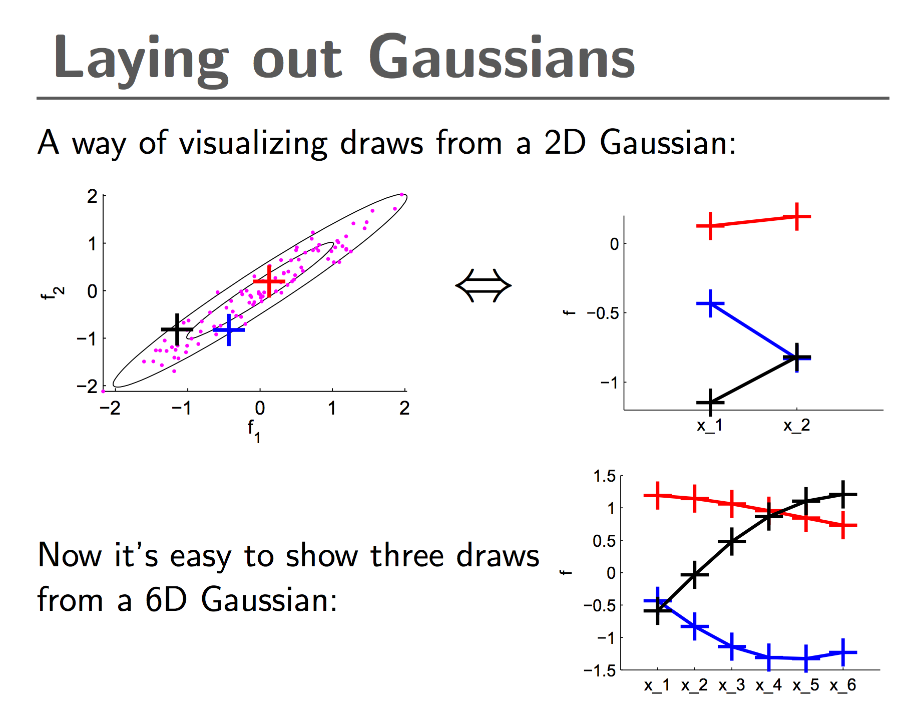
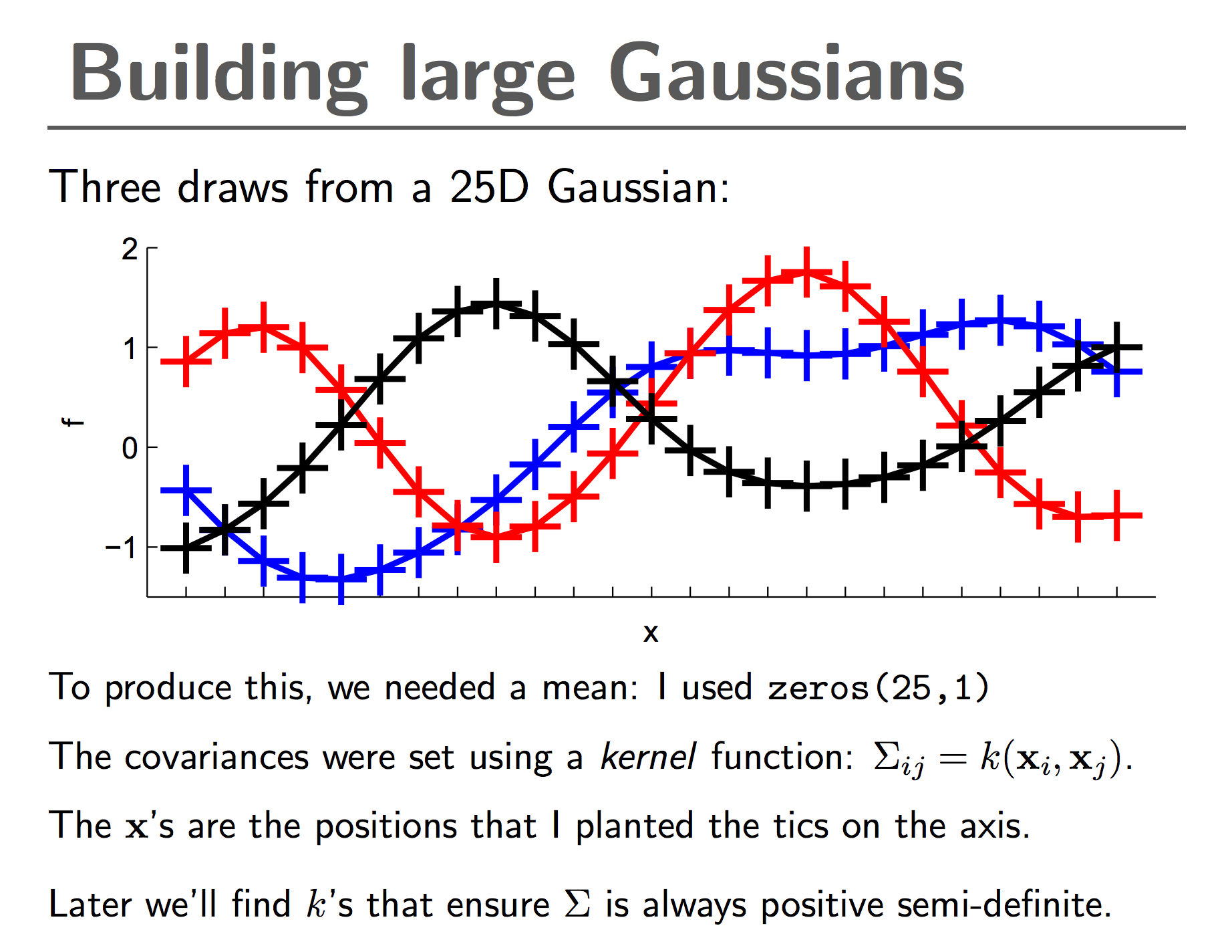
I'll be drawing $n$ samples from an $n$-dimensional gaussian distribution that is correlated. I want the correlation between $x_i$ and $x_j$ to be large for $i \approx j$ and larger as the difference between $i$ and $j$ increases. We can then look at this generated data as if it is a time-series.
Generating from Entropy
To generate this data I'll need a symmetric function rbf to create the covariance matrix for the gaussian.
$$ f(x_i, x_j) = c e^{\frac{(x_i - x_j)^2}{s}}$$
Note that the values for $c$ and $s$ can be regarded as some constant which aren't too important for the purpose of generating features. The important aspect is the symmetry. Let's do a quick for-loop to build this.
k <- 100
covmat <- matrix(0, k, k)
diag(covmat) <- 1
rbf <- function(x_i, x_j) exp(-0.5*(x_i - x_j)^2)

for(i in 1:k){
  for(j in 1:k){
    covmat[i,j] <- rbf(i/10, j/10)
  }
}
This diagonal matrix can now be used to generate random sequences.
n_guassians <- 5
df <- MASS::mvrnorm(n = n_guassians, mu = rep(0,k), Sigma=covmat) %>%
  t %>%
  data.frame %>%
  gather(key, value) %>%
  group_by(key) %>%
  mutate(r = row_number()) %>%
  ungroup

pltr <- df %>% group_by(key) %>% mutate(r = row_number(), v = value %>% cumsum) %>% ungroup

ggplot() +
  geom_line(data=df, aes(r, value, colour = key)) +
  facet_grid(key ~ .) +
  ggtitle('correlated gaussian sequences')
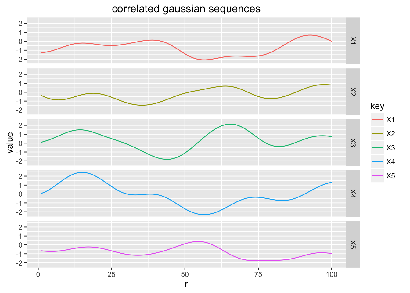
You'll notice that although these sequences are all random, they contain information. It is not white-noise, rather a biased pattern that's random enough that it cannot be predicted beforehand.
Here comes the thought experiment. If we generate enough of these 'features', can we fit these to any arbitrary continous sequenes?
n_guassians <- 5

gen_gaussians <- function(n_gauss, func){
  MASS::mvrnorm(n = n_gauss, mu = rep(0,k), Sigma=covmat) %>%
    t %>%
    data.frame %>%
    mutate(r = row_number(),
           y = func(r/10))
}

plot_datafit <- function(gauss_df){
  mod <- lm(y ~ ., data = gauss_df %>% select(-r))

  gauss_df <- gauss_df %>%
    mutate(pred = predict(mod, .))

  ggplot() +
    geom_point(data=gauss_df, aes(r, y)) +
    geom_line(data=gauss_df, aes(r, pred), colour = "steelblue") +
    ggtitle(paste("number of gaussians for fit:", (gauss_df %>% ncol) - 3))
}

show_fit <- function(n_gauss, func) {
  func %>%
    gen_gaussians(n_gauss, .) %>%
    plot_datafit
}

func1 <- function(x) sin(x/2) + 2*cos(x*2)
func2 <- function(x) 2^(sin(x/2) + 2*cos(x*2))
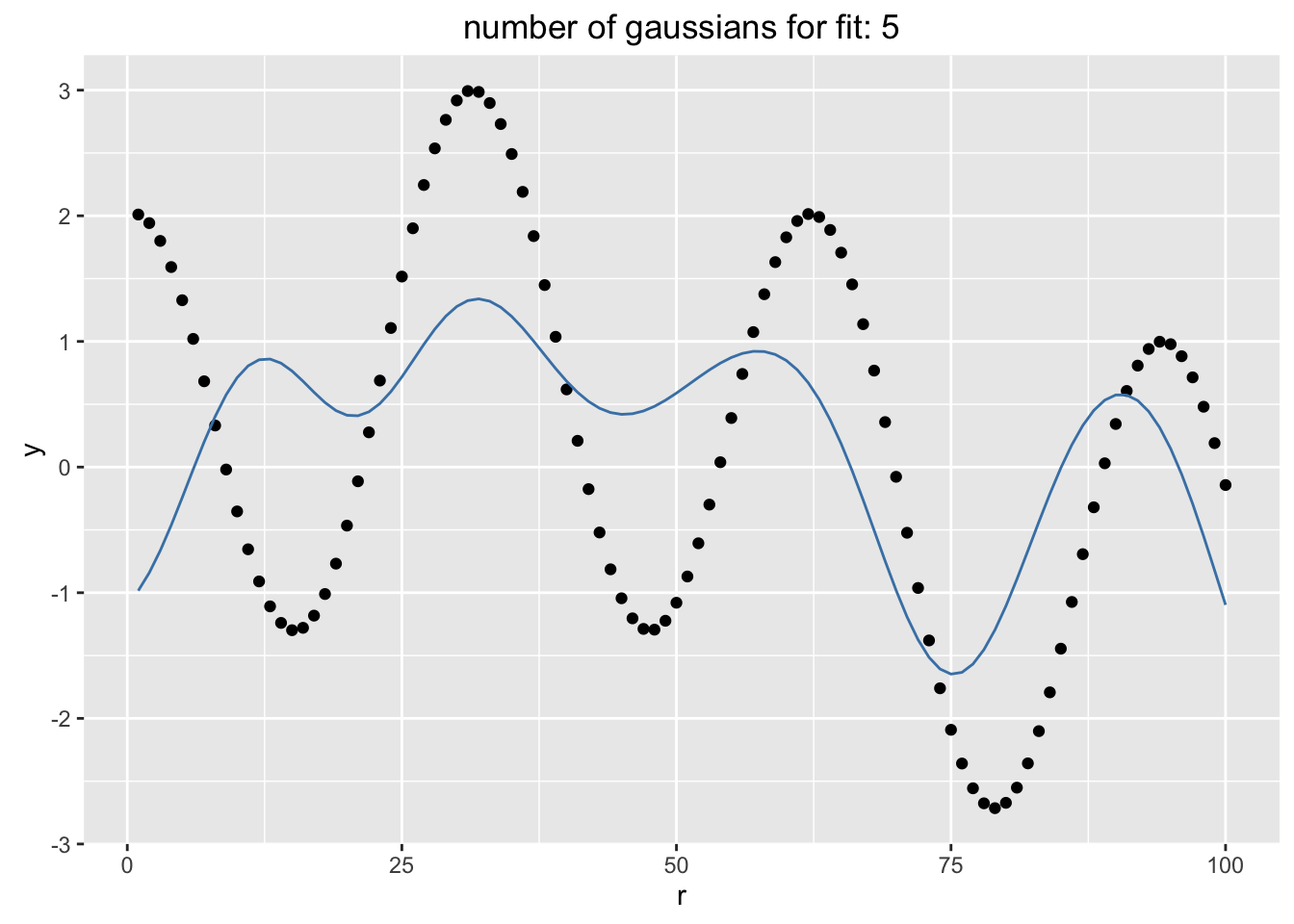
Fitting: $\sin(x/2) + 2\cos(2x)$
show_fit(5, func1)
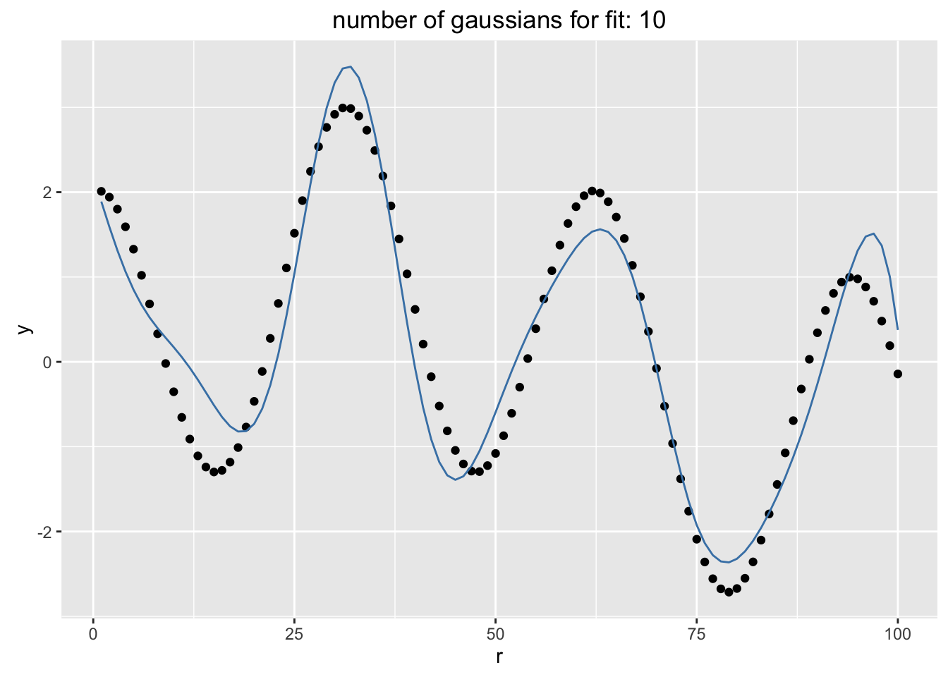
show_fit(10, func1)
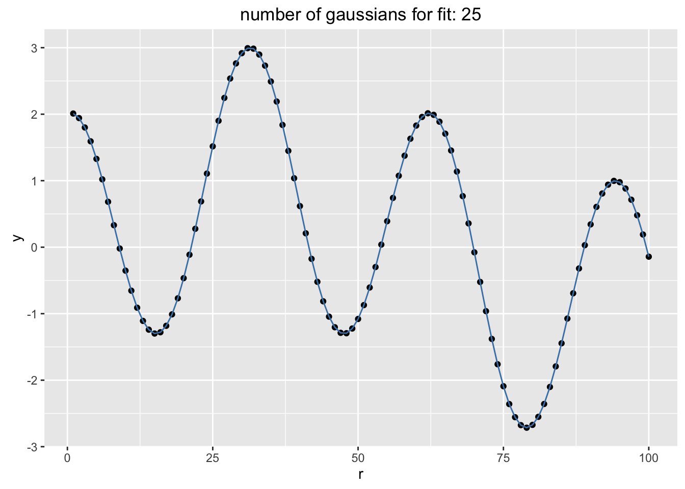
show_fit(25, func1)
Fitting: $2^{sin(x/2) + 2*cos(2x)}$
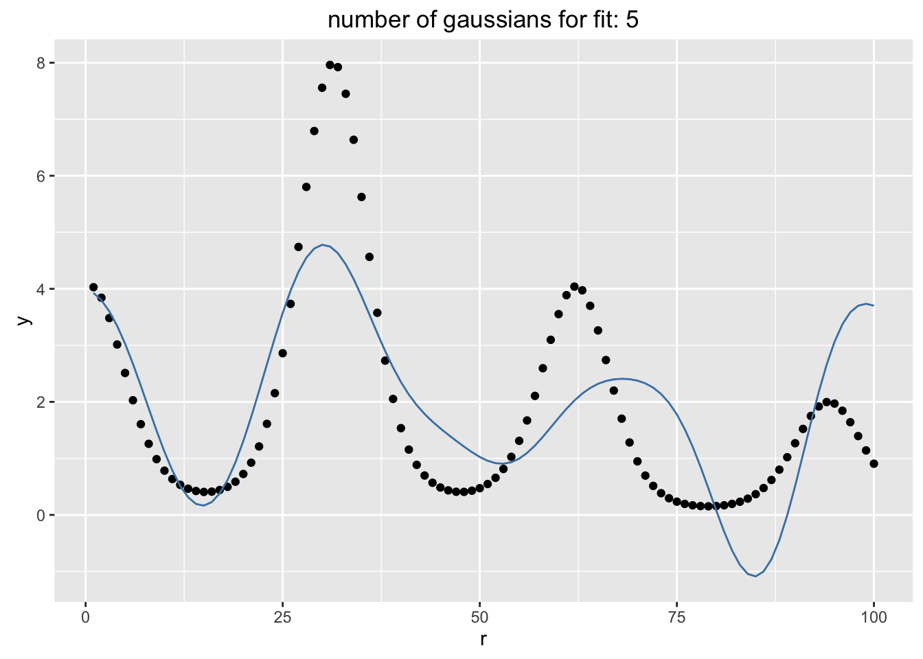
show_fit(5, func2)
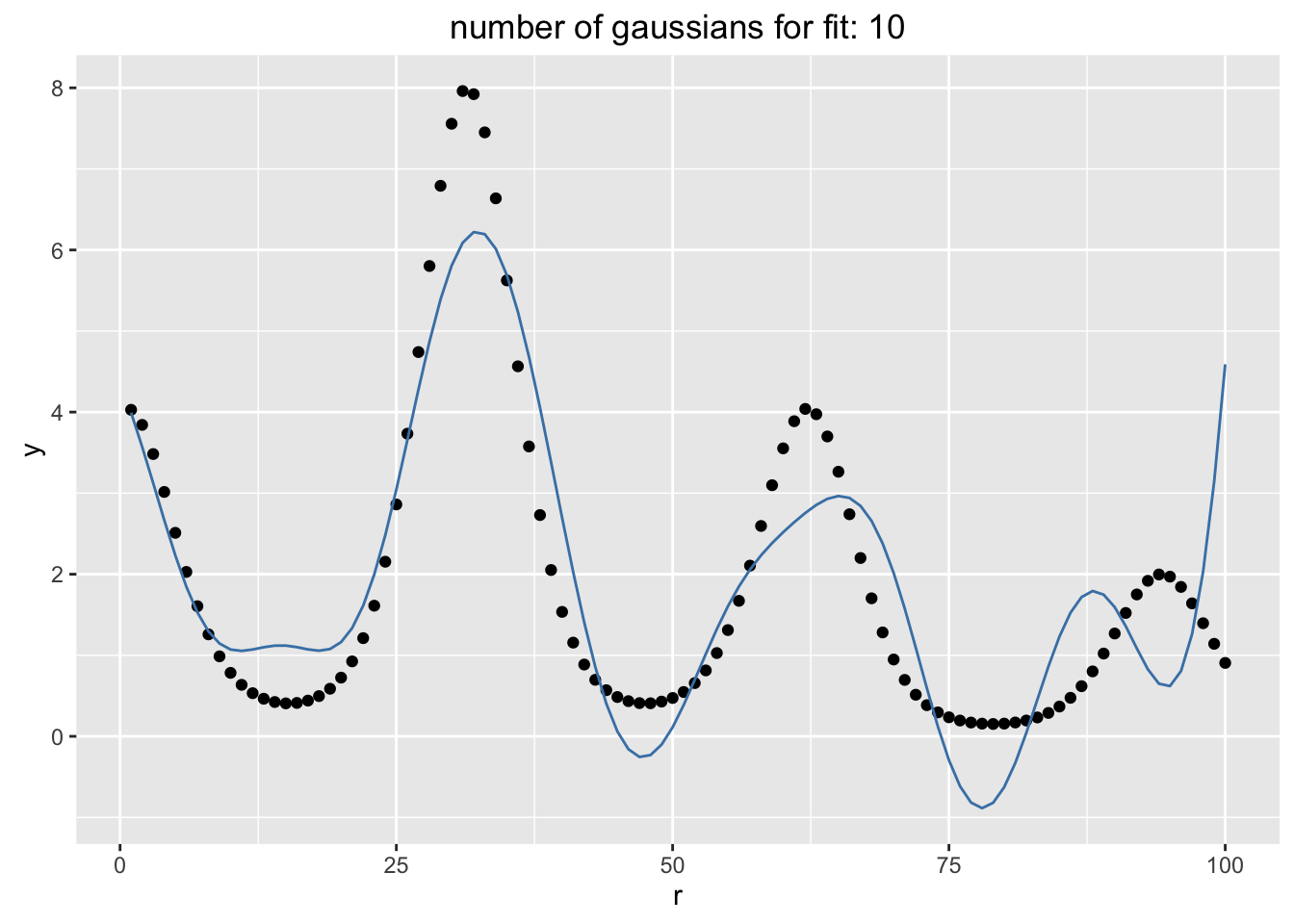
show_fit(10, func2)
show_fit(25, func2)
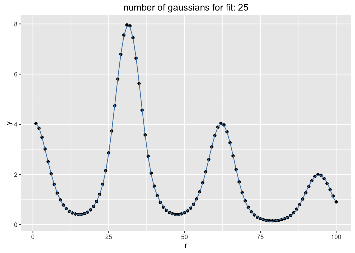
We seem to be fitting rather well. This is an interesting feat. Because we're generating smooth random patterns, we are able to find a linear combination of them that fit the data well.The resulting fit is also very smooth. In a lot of ways this process is very similar to the exercize with the radial basis functions, except here I'm able to do this with (biased) random features.
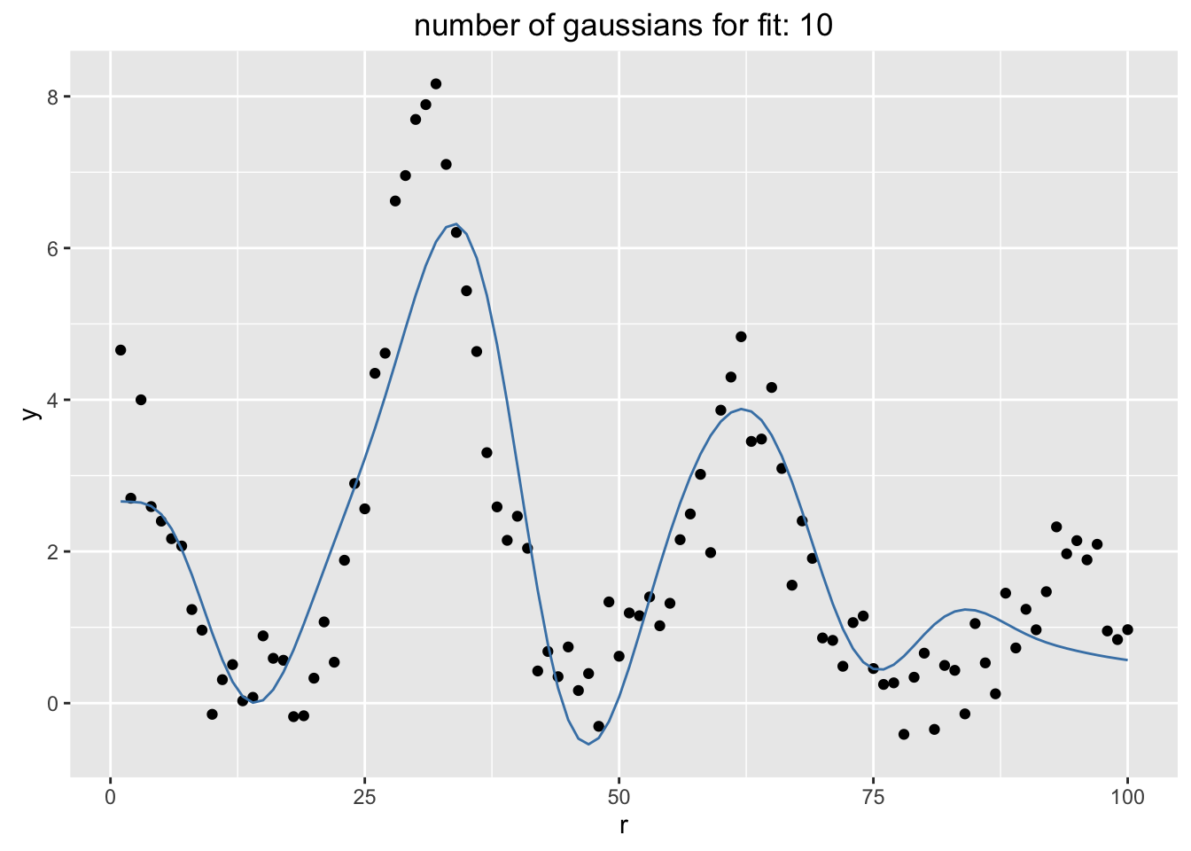
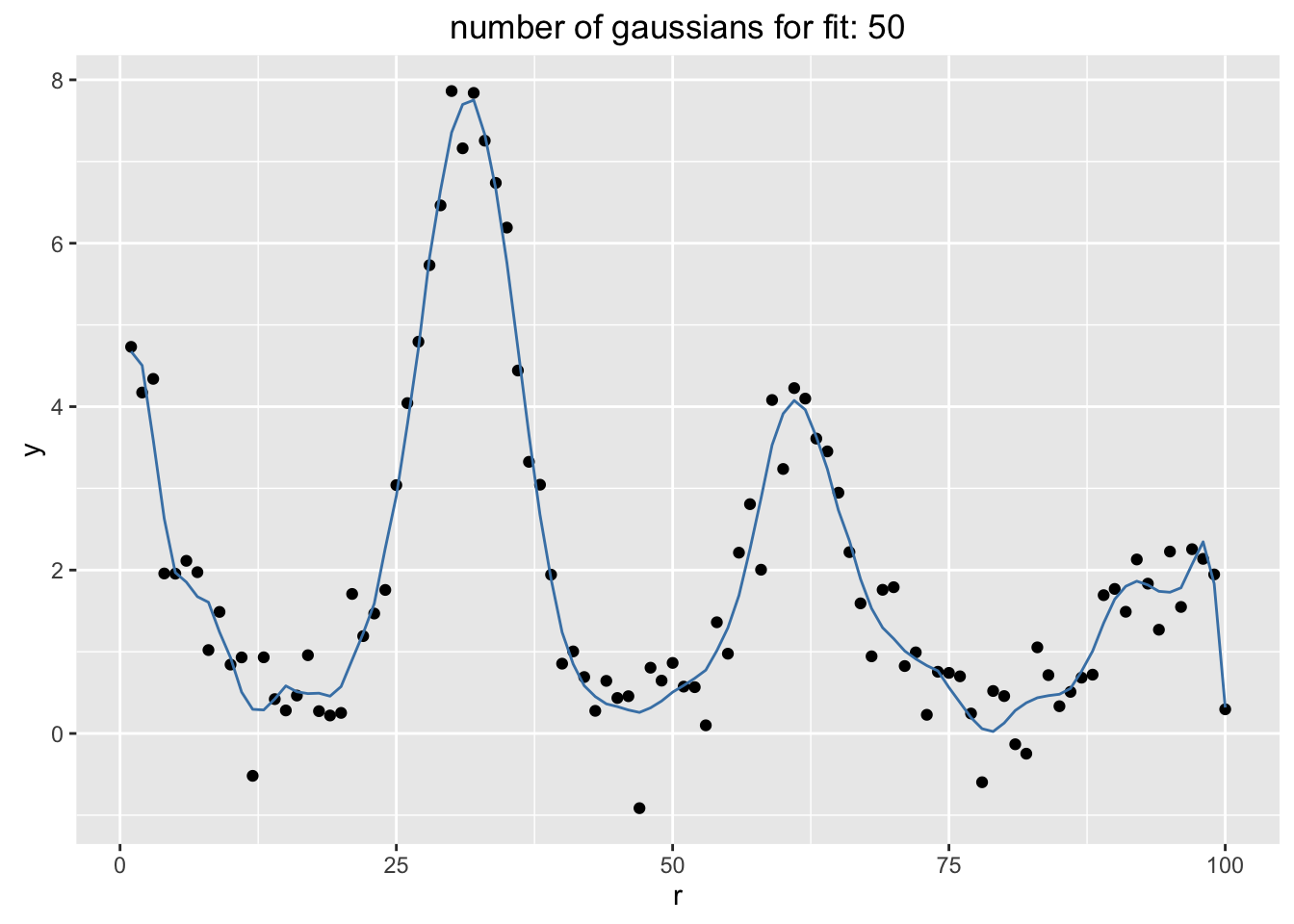
Can I haz noisy data?
Yes! Although if the signal to noise ratio is off, you can expect the fit to capture the noise more than the signal. This is expected with most machine learning approaches.
show_fit_with_true <- function(n_gauss, func, sigma = 0.5){
  p <- show_fit(n_gauss, function(x) func(x) + rnorm(length(x), 0, sigma))
  p
}
Effect of Noise in Data
show_fit_with_true(10, function(x) 2^(sin(x/2) + 2*cos(x*2)))
show_fit_with_true(50, function(x) 2^(sin(x/2) + 2*cos(x*2)))
Conclusion
This featue generating trick might remind of a similar trick with radial basis functions. What is interesting here is that we're able to generate these features from biased entropy. Deterministic patterns can be tackled with appropriate randomness.