A friend of mine once told me a 'flawless' tactic for beating the roulette game.

1. bet on black 
  - if you lose, bet on black again but now double the amount
    - if you win now, you will have not lost any money 
    - if you lose again, bet on black again but now double the amount 
      - if you win now, you will have not lost any money 
      - if you lose again, bet on black again but now double the amount 
        - if you win now, you will have not lost any money 
        - if you lose again, bet on black again but now double the amount 
          etc ... 
  - if you win, profit! 
2. repeat

The idea is that the probability of always getting red converges to zero and as of such you should always be able to win lost money back.

In this document I will explain why this tactic is flawed via probability theory as well as simulations. As a seperate goal, this document will also help explain simulation and lazy plotting patterns in R.

Simulating Gambles in R

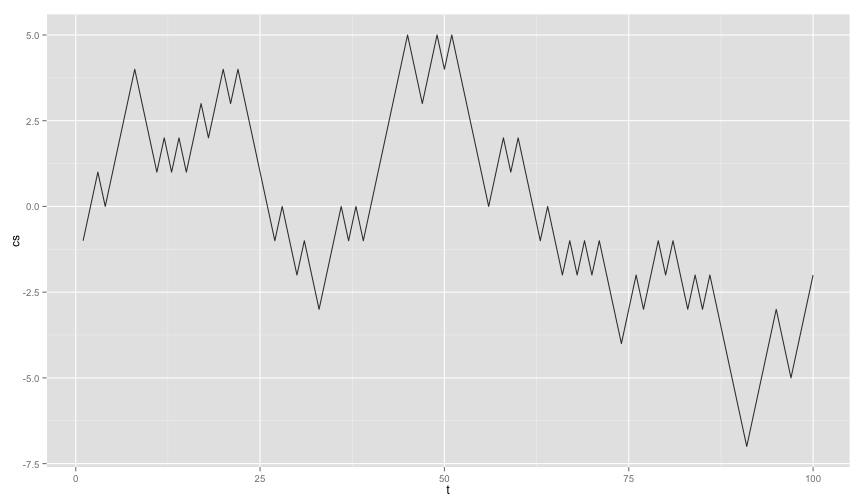
Let's start by first simulating and drawing a random path. For these first simulations we will assume that everytime you gamble you win some or lose some depending on the output of a cointoss. A possible way of simulating this can be via;

randints = function(num) {
    sample(c(-1, 1), num, replace = TRUE)
}

df1 = data.frame(cs = cumsum(randints(100)), t = 1:100)
ggplot() + geom_line(data = df1, aes(t, cs), alpha = 0.8)

gr1

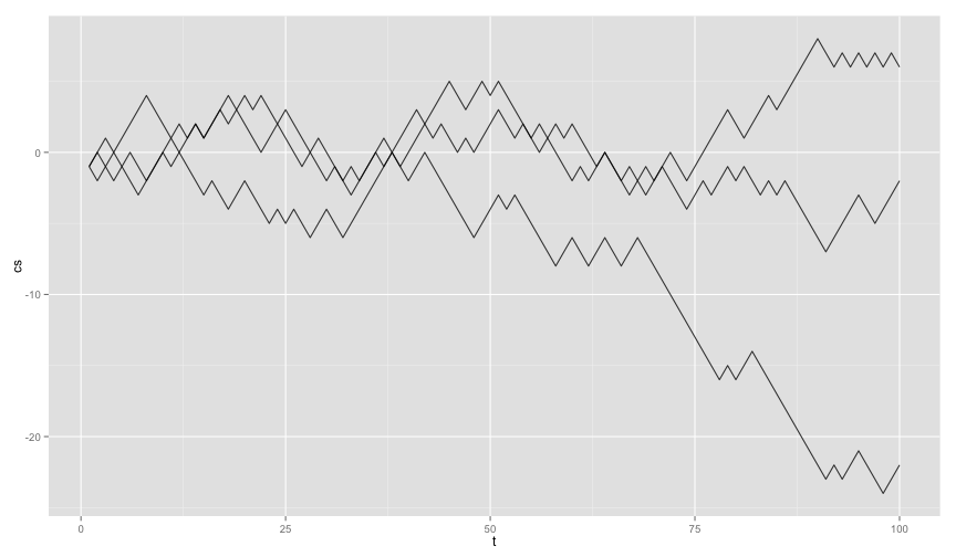
Simulating another such line and adding that to the plot is straightforward.

df2 = data.frame(cs = cumsum(randints(100)), t = 1:100)
df3 = data.frame(cs = cumsum(randints(100)), t = 1:100)
ggplot() + geom_line(data = df1, aes(t, cs), alpha = 0.8) + geom_line(data = df2, 
    aes(t, cs), alpha = 0.8) + geom_line(data = df3, aes(t, cs), alpha = 0.8)

gr2

The code can be made more elegant by exploiting the lazy evaluation of the ggplot2 library. You don't need to write a single line of ... + geom_line() + geom_line() + ... code. You can append it to a variable instead.

df3 = data.frame(cs=cumsum(randints(100)), t=1:100)
p = ggplot() 
p = p + geom_line(data=df1, aes(t,cs), alpha=0.8, color="red") 
p = p + geom_line(data=df2, aes(t,cs), alpha=0.8, color="green")
p = p + geom_line(data=df3, aes(t,cs), alpha=0.8, color="blue")
p

gr3

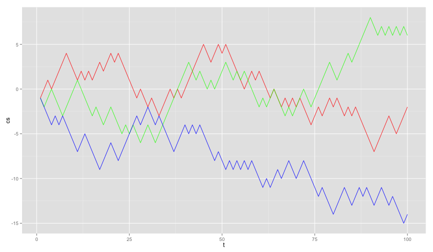
This is a more favorable pattern. You can keep adding plotting layers (from different datasets) to the variable p and it will not draw a single pixel until you call p at the end. It is clear for a user to see, line by line, that new layers are being added to the layer and you can use this pattern within a forloop. This means that you can do many simulations and draw them from a single function.

gamble_plot = function(nruns){
  p = ggplot()  
  for(i in 1:nruns){
    df = data.frame(cs=cumsum(randints(100)), t=1:100)
    p = p + geom_line(data=df, aes(t,cs), alpha=0.1)
  }
  p
}

gamble_plot(300)

gr4

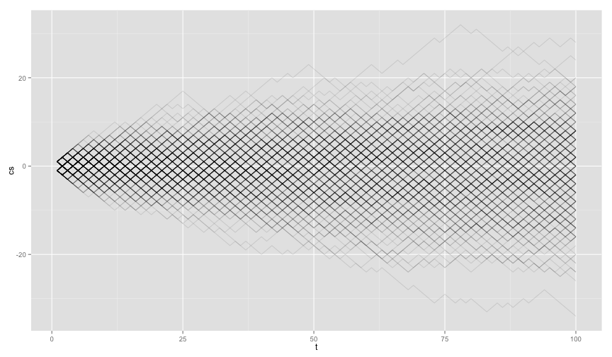
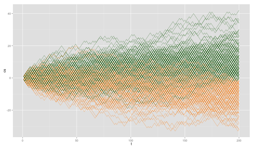
In this pattern it is also relatively easy to assign colors to series of gamblers if they result in a long term profit or loss. Also, it might make sense to have the length of the random path be an input for our simulation function.

gamble_plot = function(nruns, len){
  p = ggplot()  
  for(i in 1:nruns){
    color = "darkgreen"
    df = data.frame(cs=cumsum(randints(len)), t=1:len)
    if(select(df, cs)[len,] < 0) color = "darkorange"
    p = p + geom_line(data=df, aes(t,cs), alpha=0.4, color=color)
  }
  p
}

gamble_plot(300, 200)

gr5

Casino Royale

Using this plotting pattern, let's simulate the results from the 'flawless' roulette tactic. The following functions help the simulation.

gamble = function(moneyin){
  if( runif(1) < 0.5 ) return(moneyin) # result is black
  -moneyin # result is red
}

nextm = function(gamble, outcome){
  if(outcome < 0) return(2*gamble) #on lose we double the money
  1
}

simulate = function(maxt){
  df = data.frame(time=as.numeric(c()), money=as.numeric(c()))
  move = 0
  outcome = 0
  for(i in 1:maxt){
    move = nextm(move, outcome)
    outcome = gamble(move)
    df = rbind(df, data.frame(time=i, money=outcome))
  }
  df$money = cumsum(df$money)
  df
}

gamblersruin = function(num, maxsim){
  p = ggplot() 
  for(i in 1:num){
    df = simulate(maxsim)
    p = p + geom_line(data=df, aes(time,money), alpha=0.3)
  }
  p
}

Notice that I am assuming the probability of getting black ( $p_B$ ) and the getting ( $p_R$ ) to be equal to $0.5$ for now. This is not how a casino would play roulette but we will use it as an upper bound. If I can show that in this optimistic version of roulette the outcome of this tactic is doubtful then it will surely fail in a more realistic roulette game. Later we will also consider a more realistic roulette game.

Let's run some results.

set.seed(1)
gamblersruin(1,100) + ggtitle('single simulation, 100 bets')
gamblersruin(1,1000) + ggtitle('single simulation, 1000 bets')
gamblersruin(1,10000) + ggtitle('single simulation, 10000 bets')

gr6 gr7 gr8

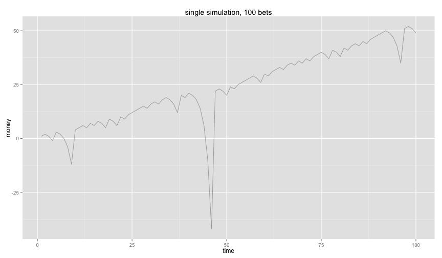
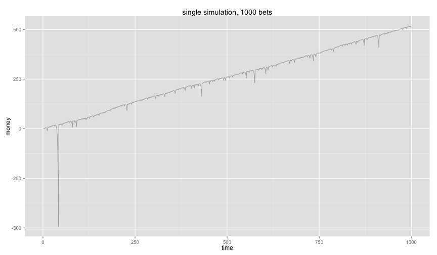
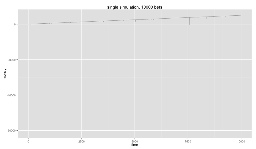
Ouch, on the long term it does seem like you are making a net profit but you are not without risk. The probability of getting red 12 times in a row is small but when you are playing this game for a very long time then this event suddenly becomes likely. And when it happens you need to compensate with $2^{12}$ cash.

Probability Theory

So the simulations are giving us reasons to be pessimistic about the tactic, but the long term end result does seem to be positive. What does mathematics tell us?

I will be a bit formal here, but thats a given when dealing with math. Suppose that we play the roulette game until we have made a profit of 0 or 1. Let's consider this outcome to be a stochastic variable $G$ . Note that a single game $G$ can have multiple bets.

Then also let $p_B$ be the probability for getting black, $p_R$ the probability for getting red, $s_B$ the payout for getting the state of black and $s_R$ the payout for getting the state of red.

𝔼 (G) = p B s B + p R s R = 1 2 + \sum k = 1 \infty p k - 1 R p B \times 0 = 1 2

$\begin{aligned} \mathbb{E}(G) & = p_Bs_B + p_Rs_R = \frac{1}{2} + \sum_{k=1}^\infty p_R^{k-1} p_B \times 0 = \frac{1}{2} \ \end{aligned}$

𝔼 (G 2) = p B s 2 B + p R s 2 R = 1 2 + \sum k = 1 \infty p k - 1 R p B \times 0 = 1 2

$\begin{aligned} \mathbb{E}(G^2) & = p_Bs_B^2 + p_Rs_R^2 = \frac{1}{2} + \sum_{k=1}^\infty p_R^{k-1} p_B \times 0 = \frac{1}{2}\ \end{aligned}$

The variance of the game is then defined via the definition.

V a r (G) = 𝔼 (G 2) - (𝔼 (G)) 2 = 1 2 - [1 2] 2 = 1 4

$\begin{aligned} Var(G) & = \mathbb{E}(G^2) - \left(\mathbb{E}(G)\right)^2 = \frac{1}{2} - [\frac{1}{2}]^2 = \frac{1}{4}\ \end{aligned}$

So what happens when we play this game an infinite amount of time?

lim n \to \infty 𝔼 (n G) = lim n \to \infty n 2 = \infty

$\lim_{n\to\infty} \mathbb{E}(nG) = \lim_{n\to\infty} \frac{n}{2} = \infty$

lim n \to \infty V a r (n G) = lim n \to \infty \sum i = 1 n V a r (G) = \infty

$\lim_{n\to\infty} Var(nG) = \lim_{n\to\infty} \sum_{i=1}^n Var(G) = \infty$

This could feel very curious but should come with no suprise. If we play the game an infinite amount of time we will have an infinite amount of risk. In laymans terms, if you want to earn an infinite amount of money you will need an infite amount of money.

Gamblers Fail

Even if we assume that you have an infinite amount of betting money, the tactic will still fail in real life. The main reasons is that casinos tend to apply a maximum bet in all their gambling games. You can never bet above a certain amount in the casino which means that you cannot apply the 'doubling' tactic infinetely.

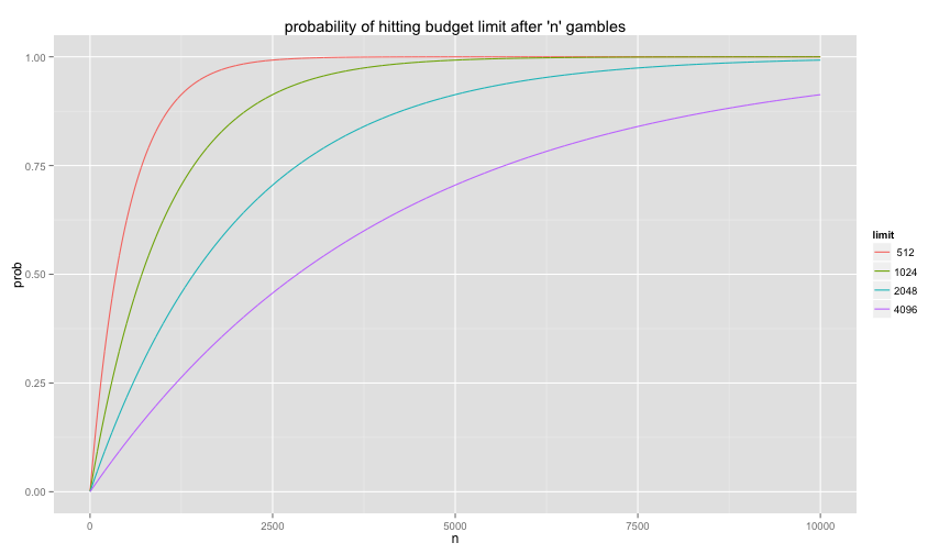
How likely is it to hit a casino limit during a game? Let $k$ be the number of sequential losses in a game and let $n$ be the number of bets played. Then the probability of having no losses in one game is defined by the following.

ℙ (no loss in 1 game) = 1 - ℙ (loss in 1 game) = 1 - 1 2 k = 2 k - 1 2 k

$\mathbb{P}(\text{no loss in 1 game}) = 1 - \mathbb{P}(\text{loss in 1 game}) = 1 - \frac{1}{2^k} = \frac{2^k - 1}{2^k}$

This can then be expanded to playing $n$ games.

ℙ (at least one loss in n games) = ℙ (no loss in n games) = 1 - (2 k - 1 2 k) n

$\mathbb{P}(\text{at least one loss in n games}) = \mathbb{P}(\text{no loss in n games}) = 1 - \left( \frac{2^k-1}{2^k} \right)^n$

Notice that you cannot play the game for an infinite amount of time now without risking such a loss.

lim n \to \infty 1 - (2 k - 1 2 k) n = 1, \forall k \geq 1

$\lim_{n\to\infty} 1 - \left( \frac{2^k-1}{2^k} \right)^n = 1, \forall k \geq 1$

f = function(k,n){
  1 - ( (2^k - 1) / ( 2^k ) )^n
}

df = data.frame(prob=f(9,1:10000), n=1:10000, limit=" 512")
df = rbind(df, data.frame(prob=f(10,1:10000), n=1:10000, limit='1024'))
df = rbind(df, data.frame(prob=f(11,1:10000), n=1:10000, limit='2048'))
df = rbind(df, data.frame(prob=f(12,1:10000), n=1:10000, limit='4096'))

p = ggplot()
p = p + geom_line(data=df, aes(n, prob, colour=limit))
p + ggtitle("probability of hitting budget limit after 'n' gambles")

gr9

Also notice that if we consider the casino bounds then the expected value of the game $G$ we defined earlier suddenly becomes zero.

𝔼 (G) = p B \times 1 - p B p R k - 1 2 k - 1 = 1 2 - 1 2 = 0

$\mathbb{E}(G) = p_B \times 1 - p_B{p_R}^{k-1} {2}^{k-1} = \frac{1}{2} - \frac{1}{2} = 0$

This conclusion changes further if we stop assuming that $p_B = p_R = 0.5$ . In the more realistic casino game (by also considering the number 37 to the casino board) the expected value would now become:

𝔼 (G) = p B \times 1 - p B p R k - 1 2 k - 1 = 0.4865 - 0.5135 = - 0.027

$\mathbb{E}(G) = p_B \times 1 - p^B{p_R}^{k-1} {2}^{k-1} = 0.4865 - 0.5135 = -0.027$

Including Fail in Simulations

Let's run some more simulations again with these facts in mind.

nextm = function(gamble, outcome){
  if(outcome < 0){
    if(gamble > 500){
      return(1)
    }
    return(2*gamble)
  }
  1
}

gamble = function(moneyin){
  if( runif(1) < 0.4865 ) return(moneyin) # result is black
  -moneyin # result is red
}

gamblersruin(50,2500) + ggtitle("50 more realistic simulations")

gr10

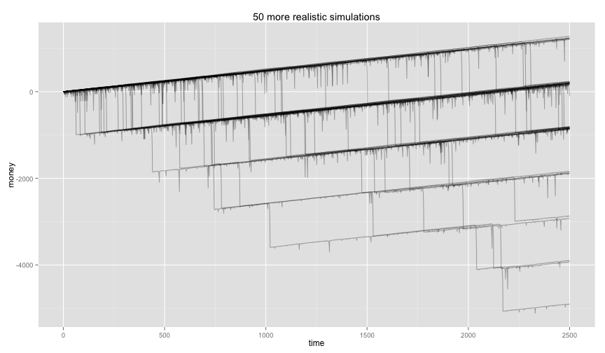
And we can see that these outcomes seem to spread out. Making a histogram of the endgame states shows us how flawed the tactic really is.

gamblersend = function(num, maxsim){
  df = data.frame(time=as.numeric(c()), money=as.numeric(c()))
  for(i in 1:num){
    if( i %% 5 == 0 ){
      cat(i, 'simulations have now run\n')
    }
    df = rbind(df, simulate(maxsim)[maxsim,])
  }
  df
}

ends = gamblersend(200,2500) # big simulation, warning, takes long
p = ggplot() 
p = p + geom_histogram(data=ends, aes(money), alpha=0.9, binwidth=1000)
p + ggtitle("histogram of casino outcomes after 2500 bets")

gr11

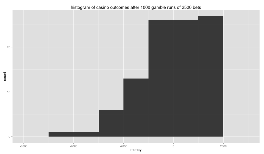
The tactic simply isn't leading to a lead positive result, we are definately making an average loss with this tactic.

> mean(ends$money)
[1] -336.2

Conclusion

These infinite betting strategies where the outcome seems riskless are known as martingales, you can find more information about them on wikipedia. Mathematics is a nice tool and should not be ignored when tackling these strategies but to confirm their flaws with something maybe a little more tangible R can be a great tool. Creating and running simulations in R is easier if you split your simulation into smaller functional bits. The lazy evaluation of ggplot can also be of help to keep the code you need clean.

You should also be able to find this blog on: r-bloggers

koaning.io

Casino Gambling Simulations in R