EDIT
The original blogpost had a gigantic error in it as discussed here. I've made improvements to the original document to reflect the corrections mentioned. When in doubt, go to reddit for honest critism. Shoutout to Penumbra_Penguin.
When I go on holiday I always bring two card games that I can play with my girlfriend: love letters and sushi go. The love letters game is especially interesting because it only consists of 16 cards which makes it fit into my jacket and I can play it literally anytime. It is fantastic to play a small card game with a coffee, overlooking a national park when it's raining. So we started playing love letters.
After a few rounds of my girlfriend not winning, she noticed that it was rather common that the same sets of cards occured after I had shuffled them. She naturally blamed me for the entire endeavor and I was left to convince her otherwise. We got into a bit of a discussion (or, argument) on how one should shuffle cards, which led me to investigate it in a python notebook.
Methods of Shuffling
I will be considering three ways of shuffling:
- the one way shuffle: the deck is kept in one hand and blocks of cards are slid unto the other hand making sure the top block of the main hand is put on top of the other hand.
- the two way shuffle: the deck is kept in one hand and blocks of cards are slid unto the other hand alternating between stacking above and below
- the noisy split shuffle: split the deck and zip the two stacks, we'll assume some noise over an otherwise perfect split.
- the human split shuffle: split the deck and zip the two stacks, we'll assume some noise over an otherwise non-perfect split.
Given these three practical methods of shuffling, which one is preferable? Also, how often does one need to shuffle?
Measurements of randomness
I will run a simulation in a bit, but I still need a measurement of preference. I will prefer the types of shuffling that give the most random stack of cards and it helps to have a method of quantifying this.
Entropy
The entropy of a distribution is defined by this formula.
$$ H[p(x)] = - \sum_i p_i \log p_i $$
The idea is that if something is unpredictable then this number should be large. There's a mathematical maximum in our situation too, if we have achieve perfect randomness (ie. each card is equally likely) then the maximum entropy only depends on the number of cards $c$in my deck.
$$ H[p(x)] = - \sum_i p_i \log p_i = - \sum_i \frac{1}{c} \log \frac{1}{c} = \sum_{i=1}^c \frac{1}{c} \log c = \log c $$
There's reason here when you think about it; the more cards in a deck, the more randomness it should have if it is properly shuffled.
In my case, I'll be calculating the entropy based of a simulation. If the entropy of the simulated $\hat{p_i}$ values is high, it should be more random.
Statistical Testing
The entropy metric feels rather formal and I wanted to play around with it because it is being used a lot in the bayesian deep learning field. After thinking about how I would solve this I figure statistical testing might just work fine here.
The probability of a card being at any index is supposed to be $\frac{1}{c}$ where $c$ is the number of cards in my deck. If I were to simulate this shuffling process say $n$ times then I could expect the total number of cards at index $i$ (which I'll refer to as $c_i$) to be distributed via;
$$ p(c_i | \text{good shuffle}) \sim \text{Binom}(n, p=\frac{1}{c})$$
Now that I determined the probability distribution, I could test for it. I could count how often I see counts of cards that are unlikely, say when $p(c_i | \text{shuffle}) < 0.01 $ or $p(c_i | \text{shuffle}) > 0.99$.
Implementation
I will need to make some assumptions on how much randomness goes on in the shuffling but I think the following bit of code simulates the situation reasonably.
class Deck:
    def __init__(self, n_cards=52):
        self.n_cards = n_cards
        self.cards = list(range(n_cards))

    def one_way_shuffle(self, n_times=1, at_a_time=[2,3,4,5,6,7]):
        cards = self.cards
        for i in range(n_times):
            new_cards = []
            num_cards = len(cards)
            i = 0
            while len(new_cards) < num_cards:
                tick_size = random.choice(at_a_time)
                new_batch, cards = cards[:tick_size], cards[tick_size:]
                new_cards = new_batch + new_cards
                i += 1
            cards = new_cards
        self.cards = new_cards
        return self

    def two_way_shuffle(self, n_times=1, at_a_time=[2,3,4,5,6,7]):
        cards = self.cards
        for i in range(n_times):
            new_cards = []
            num_cards = len(cards)
            i = 0
            while len(new_cards) < num_cards:
                tick_size = random.choice(at_a_time)
                new_batch, cards = cards[:tick_size], cards[tick_size:]
                new_cards = new_cards + new_batch if i % 2 == 0 else new_batch + new_cards
                i += 1
            cards = new_cards
        self.cards = new_cards
        return self

    def split_shuffle(self, n_times=1, p_flip=0, split_noise=0):
        for i in range(n_times):
            split_idx = round(self.n_cards/2) + random.choice(list(range(-split_noise, split_noise)) + [0])
            top = self.cards[split_idx:]
            bottom = self.cards[:split_idx]
            larger, smaller = (top, bottom) if len(top) > len(bottom) else (bottom, top)
            for i in range(round(len(top)*p_flip)):
                idx = random.choice(range(len(top)))
                old_cards = self.cards[:]
                old_cards[idx], old_cards[idx-1] = old_cards[idx-1], old_cards[idx]
                self.cards = old_cards
            for i in range(round(len(bottom)*p_flip)):
                idx = random.choice(range(len(bottom)))
                old_cards = self.cards[:]
                old_cards[idx], old_cards[idx-1] = old_cards[idx-1], old_cards[idx]
                self.cards = old_cards
            # because the top is bigger, i can do this
            if random.random() < 0.5:
                self.cards = reduce(add, [[a] + [b] for a,b in zip(larger, smaller)]) + larger[len(smaller):]
            else:
                self.cards = reduce(add, [[b] + [a] for a,b in zip(larger, smaller)]) + larger[len(smaller):]
        return self

    def shuffle(self, typename, *args, **kwargs):
        if typename == "one_way":
            return self.one_way_shuffle(*args, **kwargs)
        if typename == "two_way":
            return self.two_way_shuffle(*args, **kwargs)
        if typename == "human_noisy_split":
            return self.split_shuffle(*args,**kwargs, p_flip=0.5, split_noise=6)
        if typename == "noisy_split":
            return self.split_shuffle(*args,**kwargs, p_flip=0.7)
        assert False
You'll notice that my implementation makes a few assumptions. For the one/two-way shuffle I assume that the blocks of cards moved are between 2-7 cards each. The split shuffle assumes some sort of flip probability that determines that two cards aren't perfectly separated. In my simulation I assume that this flip probability is 10%.
Results
If create some GIFs for all three shuffling tactics. Every iteration of the gif is another shuffle. On the X-axis you see the index of cards we had before the shuffle and on the Y-axis you see the index of the shuffled deck. The resulting heatmap is the average simulation output. You can see the statistical results listed in the title, but the gif itself explain the transformations the best.
You might want to refresh the page if you want the GIFs to sync, only refresh when all GIFs have loaded.
A few observations:
- The oneway shuffle and the nonrandom split shuffle have a lot of determinism in them which ruins the randomness.
- If there wasn't any noise in the split shuffle it would be completely predictable and you might see that the deck might get back to it's original form.
- Entropy seems like a poor metric for what I'm trying to measure. By just eyeballing I can see examples of a non-random distributions appear even though the entropy is very close to maximum. This is due to the fact that entropy is an average of a $\log$ value but also due to the fact that I'm more interested in a test.
- It seems that the best way for this example to compare two distributions was to come up with a metric that involves a statistical test. The luxury I had here was that I know the distribution what I am supposed to fit, which isn't the luxury that you might have for general probability distributions. Still, I had expected entropy to be less of a vanity metric here. KL divergence also doesn't seem interesting because it would essentially boil down to the same metric.
- When just looking at these GIFs, you get the impression that the two way shuffle looks valid and very fast in randomness.
The Giant Mistake
At this point in time, you might be tempted to consider the two-way shuffle to be a winner (I certainly was; it seemed random and there's no need to bend cards). But we've been chasing a bit of a vanity metric sofar.
Consider the following shuffle technique: split the deck randomly and place the bottom deckpart on top. Is this a random shuffle? No! Might this method of shuffling pass our method of checking? Yes! If you consider the original place of card $i$ it is very hard to predict the next place where it will appear. But the card $i$ will most likely be next to card $i+1$.
The GIFs that I've shown represent a view of randomness, but merely one view. If you want to check for proper randomness you'd need to look a lot deeper and at more things than just location of the card in the deck. In particular let's look instead to the distribution of bigrams for every method of shuffling.
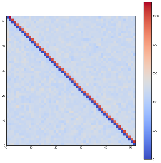
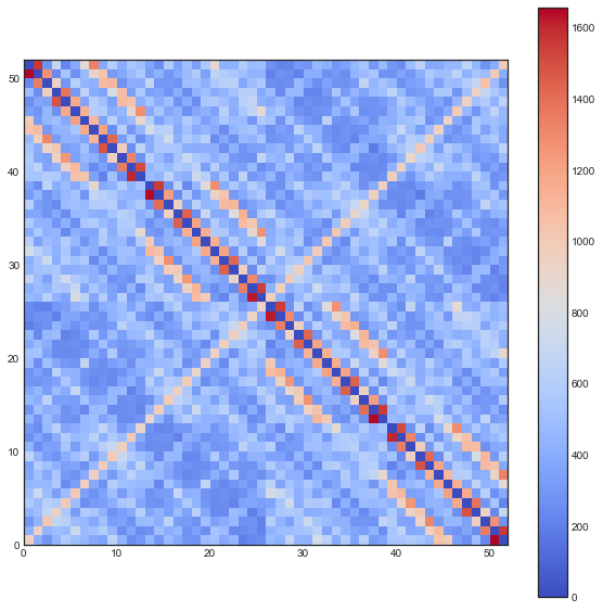
The following plots are plots of bigrams. The count value at $(x,y)$ shows how often card the card combination occured. If the count is high for $(5,6)$ for example then card 5 occurs every often just in front 6. A good shuffling algorithm would have zeros on the diagonal and flat values everywhere else. All plots below are bigram counts after 16 times of shuffling.
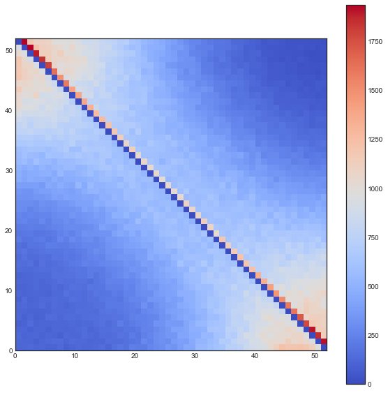
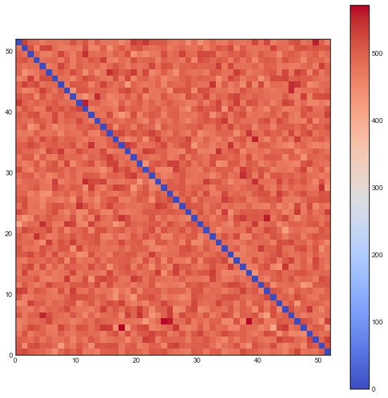
- The one-way shuffle is still a bad shuffle, also by this metric.
- The two-way shuffle, suddenly, is showing it's true colors. The diagonal is fine, but pay attention to the indices just above it. It seems this shuffling keeps the original order intact. Even though you cannot predict where the cards will be, you can predict that cards will follow suit.
- Because the deck is split perfectly every time you loose a lot of noise.
- When you let this go, it looks a whole lot better.
If you want to check the notebook for all this work check here.
Conclusion
A test can proove the existence of an error but cannot proove the absense of one. The bigram metric view is an improvement but isn't perfect.
Despite the hours spent on getting the GIFs to work, I couldn't proove my girlfriend wrong and she's now fully convinced that I'm cheating. I still think my efforts were fruitful though. When playing a card game, two way shuffling is a bad method of shuffling. Split shuffling works but only if you add plenty of randomness yourself. It seems that shuffling about 7 times should be fine.