In this document I will demonstrate density mixture models. The goal for me was to familiarize myself with tensorflow a bit more but it grew to a document that compares models too. The model was inspired from this book by Christopher Bishop who also wrote a paper about it in 1994. I'll mention some code in the post but if you feel like playing around with the (rather messy) notebook you can find it here.

Density Mixture Networks

A density mixture network is a neural network where an input $\mathbf{x}$ is mapped to a posterior distribution $p(\mathbf{y} | \mathbf{x})$. By enforcing this we gain the benefit that we can have some uncertainty in our prediction (assign a lot of doubt for one prediction and a lot of certainty for another one). It will even give us the opportunity to suggest that more than one prediction is likely (say, this person is either very tall or very small but not medium).

The main trick that facilitates this is the final hidden layer which can be split up into three different parts:

• a $\boldsymbol{\mu}$ layer with nodes ${\mu_1 ... \mu_k}$ which will denote the mean of a normal distribution
• a $\boldsymbol{\sigma}$ layer with nodes ${\sigma_1 ... \sigma_k}$ which will denote the deviation of a normal distribution
• a $\boldsymbol{\pi}$ layer with nodes ${\pi_1 ... \pi_k}$ which will denote the weight of the associated normal distribution in the resulting prediction

The idea is that the final prediction will be a probability distribution that is given by the trained output nodes via;

$$ p(\mathbf{y} | \mathbf{x}) = \sum_{i=1}^k \pi_i \times N(\mu_i, \sigma_i) $$

Graphically, and more intuitively, the network will look something like:

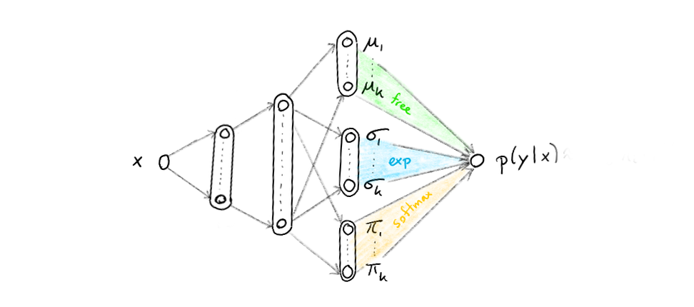
All the non-coloured nodes will have tahn activation functions but to ensure that the result is actually a probability distribution we will enforce this neural network to:

1. ensure that $\sum_i \pi_i = 1$ at all times, we can use a softmax activation to enforce that
2. ensure that every $\sigma_i > 0$, we can use an exponential activation to enforce that

Note that the architecture we have is rather special. Because we assign nodes to probibalistic meaning we enforce that the neural network gets some bayesian properties.

Implementation

The implementation is relatively straightforward in tensorflow. To keep things simple, note that I am using the slim portion of contrib.

import tensorflow as tf 

# number of nodes in hidden layer
N_HIDDEN = [25, 10]
# number of mixtures
K_MIX = 10

x_ph = tf.placeholder(shape=[None, 1], dtype=tf.float32)
y_ph = tf.placeholder(shape=[None, 1], dtype=tf.float32)

nn = tf.contrib.slim.fully_connected(x_ph, N_HIDDEN[0], activation_fn=tf.nn.tanh)
for nodes in N_HIDDEN[1:]:
    nn = tf.contrib.slim.fully_connected(nn, nodes, activation_fn=tf.nn.tanh)

mu_nodes = tf.contrib.slim.fully_connected(nn, K_MIX, activation_fn=None)
sigma_nodes = tf.contrib.slim.fully_connected(nn, K_MIX, activation_fn=tf.exp)
pi_nodes = tf.contrib.slim.fully_connected(nn, K_MIX, activation_fn=tf.nn.softmax)

norm = (y_ph - mu_nodes)/sigma_nodes
pdf = tf.exp(-tf.square(norm))/2/sigma_nodes
likelihood = tf.reduce_sum(pdf*pi_nodes, axis=1)
log_lik = tf.reduce_sum(tf.log(likelihood))

optimizer = tf.train.RMSPropOptimizer(0.01).minimize(-log_lik)
init = tf.global_variables_initializer()

Experiments

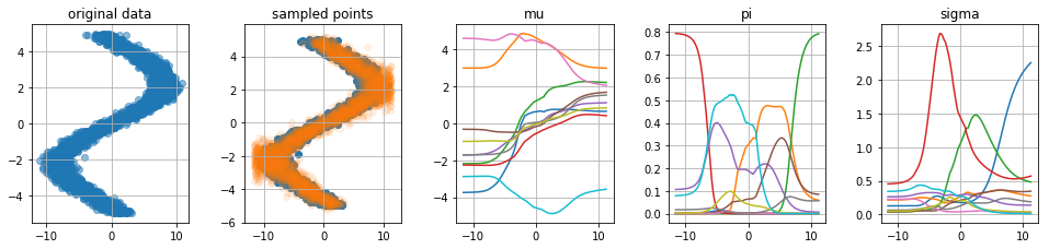
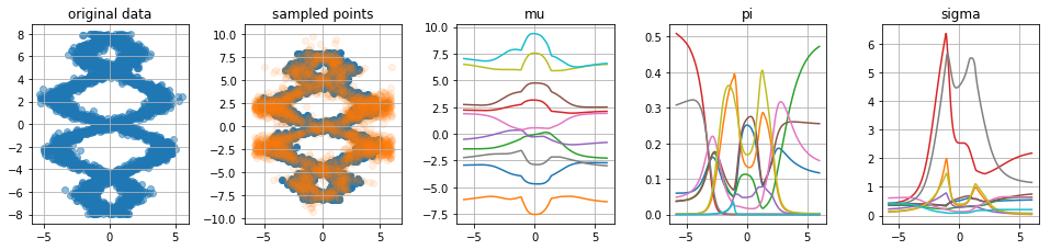
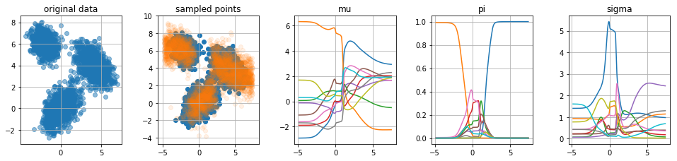
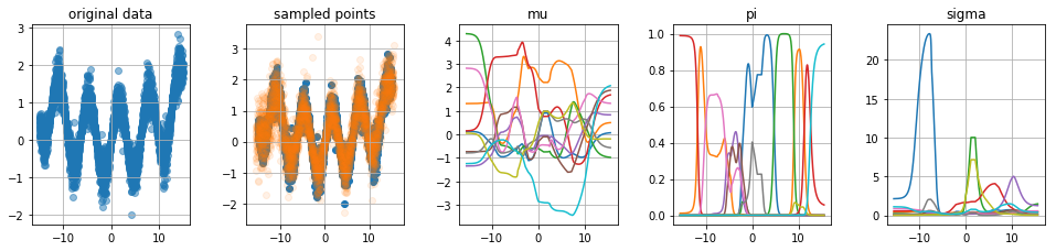
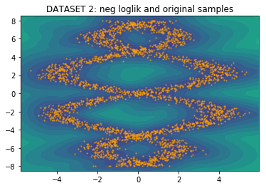
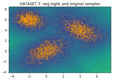
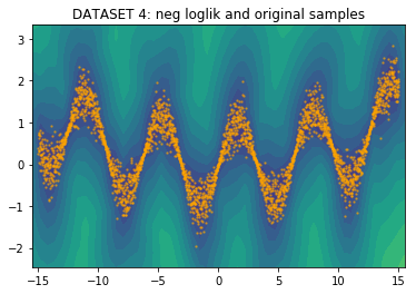
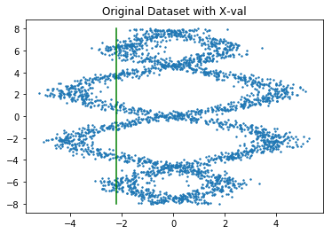
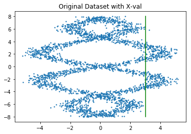
With the implementation ready, I figured it would be nice to generate a few odd datasets to see how the architecture would hold. Below you will see five charts for four datasets.

1. The first chart shows the original dataset which was sampled via numpy.
2. The second chart shows the original dataset with samples from the predicted distribution. We first sample $x$ to get the associated values at the $\boldsymbol{\mu}, \boldsymbol{\sigma}$ and $\boldsymbol{\pi}$ nodes in the network. To get a sample from $p(y|x)$ we first decide which normal distribution $N(\mu_i, \sigma_i)$ to sample from using the weights $\boldsymbol{\pi}$.
3. The third plot shows the value for the different $\mu_i$ nodes given certain values of input $x$.
4. The fourth plot shows the value for the different $\pi_i$ nodes given certain values of input $x$. Note that for every $x$ we hold that $\sum_i \pi_i = 1$.
5. The fifth plot shows the value for the different $\sigma_i$ nodes given certain values of input $x$.

Criticism

When looking at these charts we seem to be doing a few things right:

1. Our predicted distribution is able to recognize when a prediction needs to be multi-peaked
2. Our predicted distribution is able to understand area's with more or less noise
3. We can confirm that our $\mu_i$ lines correspond to certain shapes of our original data.

If you look carefully though you could also spot two weaknesses.

Weakness 1: very large sigma values

The values for sigma can suddenly spike to unrealistic heights, this is mainly visable in the fourth plot. I've introduced some regularisation to see if it helps. The model seems to improve, not just in the $\sigma$-space but also in the $\mu$-space we are able to see more smooth curves.

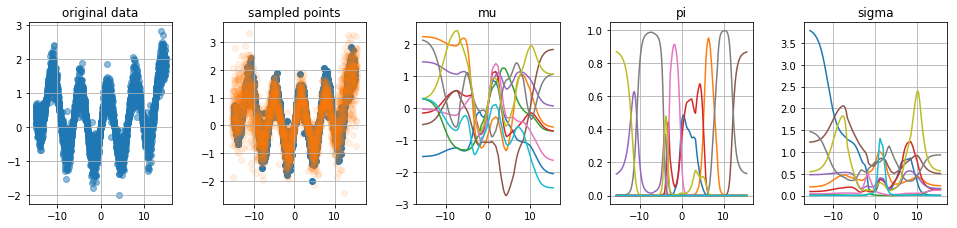
The regularisation can help, but since $\pi_i$ can be zero (which cancels out the effect of $\sigma_i$) you may need to regulise drastically if you want to remove it all together. I wasn't able to come up with a network regulazier that removes all large sigma values, but I didn't care too much because I didn't see it back posterior output (because in those cases, one can imagine that $\pi_i \approx 0$).

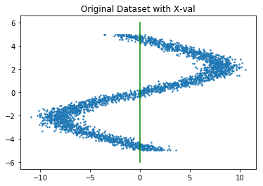
Weakness 2: samples around the edges

Our model is capable of sampling wrong numbers around the edges of the $x$-space, this is because $\sum_i \pi_i = 1$ which means that for every $x$ the likelihood must be zero. To demonstrate the extremes consider these samples from the previous models;

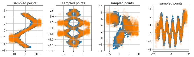
Note how the model seems to be drawing weird samples around the edges of the known samples. There's a blob of predicted orange where there are no blue datapoints to start with.

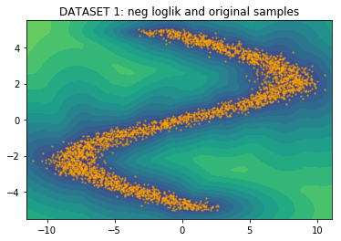
Because $\sum \pi(x) = 1$ we are always able to generate data in regions where there really should not be any. You can confirm this by looking at the $\mu$ plots. We could append this shortcomming by forcing that $\sum \pi(x) = 0$ if there is no data near $x$. We could "fix" this by appending the softmax part of the $\pi_i$ nodes with a sigmoid part.

This can be done, but it feels like a lot of hacking. I decided not to invest time in that and instead considered comparing mixture density networks to their simpler counterpart; gaussian mixture models.

Something Simple?

It is fashionable thing to try out a neural approach these days, but if you would've asked me the same question three years ago with the same dataset I would've proposed to just train a gaussian mixture model. That certainly seems like a right thing to do back then so why would it be wrong now?

The idea is that we throw away the neural network and that we train $K$ multivariate gaussian distributions to fit the data. The great thing about this approach that we do not need to implement it in tensorflow either since scikit learn immediately has a great implementation for it.

from sklearn import mixture
clf = mixture.GaussianMixture(n_components=40, covariance_type='full')
clf.fit(data)

With just that bit of code, very quickly train models on our original data too.

The model trains very fast and you get the eyeball impression that it fits the data reasonably.

Simple Comparison

Let's zoom in on predictions from both models to see how different they are.

It should be said that we'll be making comparisons between two approaches without any hypertuning (or even proper convergence checking). This is not very appropriate academically, but it may demonstrate the subtle differences in output better (as well as simulate how industry users will end up applying these models). Below we'll list predictions from both models.

In each case, we'll be given an $x$ value and we want to predict the $y$ value. The orange line is the neural approach and the blue line is from the scikit model. I've normalized both likelihoods on the same interval in order to compare them better.

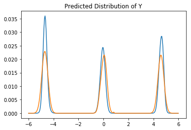
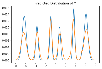
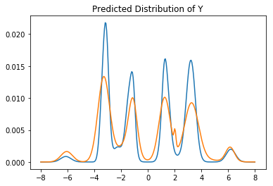
It's not exactly a full review but just from looking at this we can see that the models show some modest differences. The neural approach seems to be more symmetric (which is correct; I sampled the data that way) but it seems to suffer from unfortunate jitter/spikyness at certain places. More data/regularisation might fix this issue.

Other than that, I would argue the normal scikit learn model is competitive simply because it trains much faster which could make it feasible to do a grid search on the number of components relatively quickly.

Conclusion

Both methods have it's pros and cons, most notably;

• The neural approach takes much longer to train and you need to pay some attention to check that your model has actually converged.
• Both approaches can be tuned further but it seems the neural approach has more dials you can tweak because of the number of hidden neurons/activations.
• Picking the appropriate number of GMM components feels tricky in general, picking the appropriate hidden layer sizes feels less risky because $\pi()$ nodes can cancel out unwanted effects. One can add too many nodes/layers and still be able to live with it (albeit less ideal).
• If you sample from the neural approach from a region that does not occur in the original dataset you should expect crazy results. You will get a similar effect from a GMM if you enforce it to sample from a region of extremely low likelihood.
• The general GMM allows you to infer from $x \to y$ as well as $y \to x$ where the basic neural approach does not allow this out of the box.
• We cannot properly infer the likelihood of being at $(x,y)$ with the neural approach either because in a region where the likelihood should be near zero we still enforce $\sum_i \pi_i = 1$. So maybe we need to conjure up another network structure to accomodate this but this may require a bit of ugly hacking.
• We didn't expand to higher dimensions, but as long as we infer from $\mathbf{x} \to \mathbf{y}$ and if $y_i$ has dimension 1 our neural approach is still applicable. If this is not the case we may need to invest in encoding co-variates as well.
• One can imagine that the neural approach offers more flexibility in latent space to learn complicated relationships that might not be modelled with a mere combination of gaussians. Personally, I'm having trouble imagining an obvious example though.

Again, if you feel like playing around with the code, you can find it here.