In a previous blogpost I've discussed how sampling methods can be useful in probibalistic modelling. They will explore the parameter space such that hopefully you get a good impression of the posterior distribution. In maths, you'll most likely be able to approximate;
$$p(\theta | D)$$
But I started wondering a bit. The posterior is nice, but during prediction we may still only be interested the most likely parameters so we may be able to just go for MLE instead of doing all this sampling to find a posterior. Sampling techniques are less prone to get stuck in a local optima, but they still aren't perfect.
I got so curious I had to rewrite some code.
Switchpoint Model
I'm interested in modelling a switchpoint problem. We have an example of a timeseries with a switchpoint plotted below.
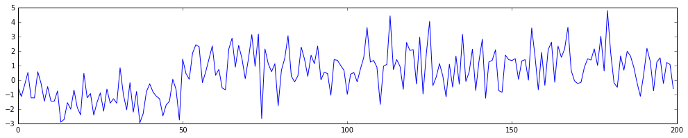
The goal for us is to find out where the changepoint is algorithmically as well as derive the mean and variance of the timeseries before and after the changepoint. In this case $\theta = { \tau, \mu_1, \mu_2, \sigma_1, \sigma_2}$, where $\tau$ is the moment in time where the switch occured, $\mu_1, \sigma_1$ correspond to the mean and variance before the switchpoint and $\mu_2, \sigma_2$ correspond to the mean and variance after the switchpoint. We are given some dataset $D$ and are therefore interested in finding;
$$ \mathbb{P}(\tau, \mu_1, \mu_2, \sigma_1, \sigma_2 | D) $$
Thanks to bayes-rule, we know the following;
\begin{aligned} \mathbb{P}(\tau, \mu_1, \mu_2, \sigma_1, \sigma_2 | D) &\propto \mathbb{P}(D | \tau, \mu_1, \mu_2, \sigma_1, \sigma_2)\mathbb{P}(s, \mu_1, \mu_2, \sigma_1, \sigma_2) \\ & = \Pi_i \mathbb{P}( y_i | \tau, \mu_1, \mu_2, \sigma_1, \sigma_2)\mathbb{P}(\tau, \mu_1, \mu_2, \sigma_1, \sigma_2) \end{aligned}
The likelihood will be defined via;
$$ \mathbb{P}( y_i | s, \mu_1, \mu_2, \sigma_1, \sigma_2) = \begin{cases} y_i \sim N(\mu_1, \sigma_1) &\mbox{if } i \leq \tau \\ y_i \sim N(\mu_2, \sigma_2) & \mbox{if } i > \tau \end{cases}$$
Now for this blogpost, I'll not be sampling. I'll merely by optimising this likelihood, which can be optimised via gradient descent on a function $f$.
$$ f(s, \mu_1, \mu_2, \sigma_1, \sigma_2) = \Pi_i \mathbb{P}( y_i | \tau, \mu_1, \mu_2, \sigma_1, \sigma_2) \approx \mathbb{P_\text{ML}}( \tau, \mu_1, \mu_2, \sigma_1, \sigma_2 | D) $$
You'll notice that I've ignored the prior for now for the sake of simplicity. I'll just focus in on the likelihood part of the equation.
Below I've added a tensorflow implementation of a gradient descent. You may notice that numerically I need to pull off a trick to implement the switchpoint. This is due to the tensorlogic of tensorflow, see here.
# tensor-check.py
import tensorflow as tf
import numpy as np

x1 = np.random.randn(35)-1
x2 = np.random.randn(35)*2 + 5
x_all = np.hstack([x1, x2])
len_x = len(x_all)
time_all = np.arange(1, len_x + 1)

mu1 = tf.Variable(0, name="mu1", dtype=tf.float32)
mu2 = tf.Variable(0, name = "mu2", dtype=tf.float32)
sigma1 = tf.Variable(2, name = "sigma1", dtype=tf.float32)
sigma2 = tf.Variable(2, name = "sigma2", dtype=tf.float32)
tau = tf.Variable(15, name = "tau", dtype=tf.float32)
switch = 1./(1+tf.exp(tf.pow(time_all - tau, 1)))

mu = switch*mu1 + (1-switch)*mu2
sigma = switch*sigma1 + (1-switch)*sigma2

likelihood_arr = tf.log(tf.sqrt(1/(2*np.pi*tf.pow(sigma, 2)))) - tf.pow(x_all - mu, 2)/(2*tf.pow(sigma, 2))
total_likelihood = tf.reduce_sum(likelihood_arr, name="total_likelihood")

optimizer = tf.train.AdamOptimizer()
opt_task = optimizer.minimize(-total_likelihood)
init = tf.global_variables_initializer()

with tf.Session() as sess:
    sess.run(init)
    for step in range(40000):
        lik, opt = sess.run([total_likelihood, opt_task])
A more advanced snippet of code can be found here which also contains bits for tensorboard. The nice thing about having a python script with tensorboard is that you can cook dinner with your partner while the computer does a lot of work while you are out there enjoying life. All you need to type is;
for i in `seq 10`; do python tensor-check.py; done
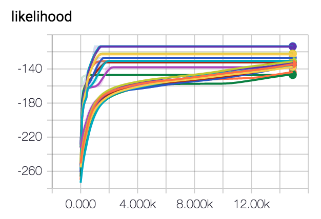
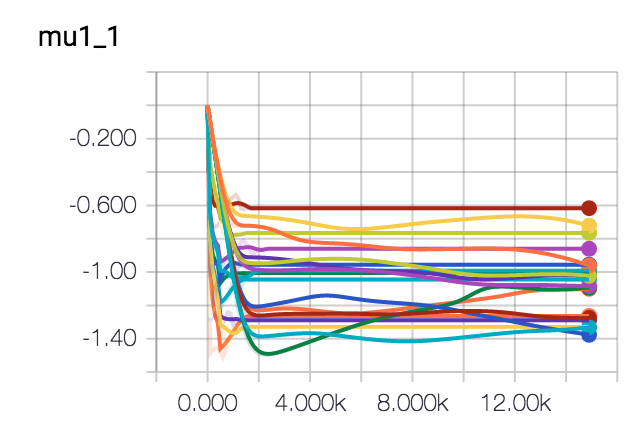
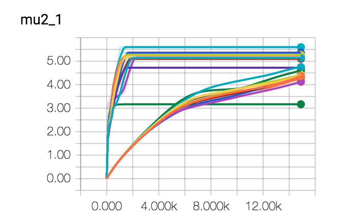
Results
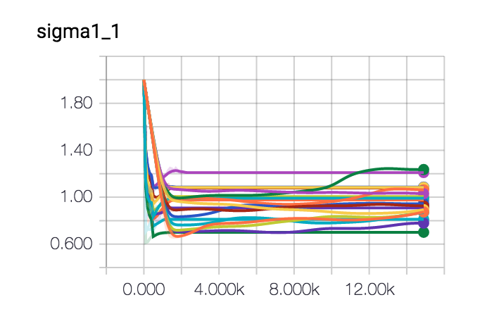
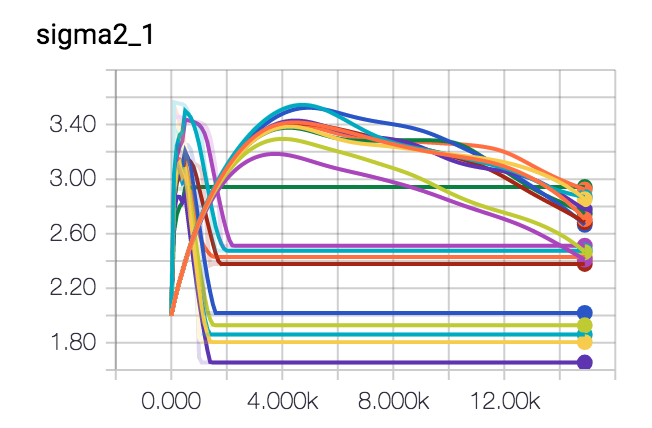
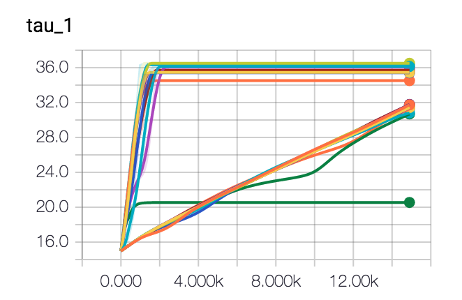
I've let this spin a few times and I've been trying out some different optimisers too. It seems like gradient descent seems to be getting us in the butterzone of the correct parameters. It may look as if it gets stuck into some form of hill but this is due to the randomness of the dataset.
Conclusion
Neither approach is perfect but it seems like the blunt gradient approach may actually also work. You'll lose information on the posterior distribution over your parameters but it may run a whole lot quicker and give you more of an impression of convergence.