In this document I'll explain a fun scraping/simulation exercize where I try to investigate the value of investing in lego minifigures. The scraping result will immediately suggest that investing in minifigures might be a profitable venture. The stochastic process behind it requires more work, but might have interesting side effects for decision theorists.
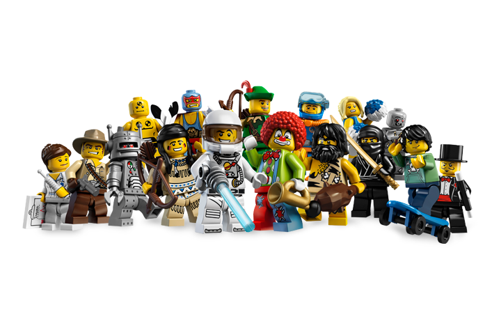
Lego Minifigures
I bought myself a simpsons minifigure for my birthday. I grabbed a shiny package, bought it and was lucky enough to get the actual Homer Simpson figure. Legos are a popular collectible and so are all things simpsons. I then went to ebay to discover that there might be a surplus in buying packages and selling complete minifigure sets.
Each set contains 16 figures and each figure costs $3. Let's download some data. We'll use common R packages.
library(purrr)
library(dplyr)
library(stringr)
library(ggplot2)
library(rvest)
library(parallel)
I've taken the liberty of acquiring some prices for full sets of lego minifigures. I've got a set of prices for a set of simpsons minifigures and a set of any lego series.
simpson_prices <- c(58.99, 59.99, 120.00, 65.00, 100.00, 74.99, 115.00, 114.95, 129.99, 60.00, 92.72, 99.87, 49.92, 55.63, 114.14, 142.67, 71.34, 57.07, 54.20, 49.22, 57.05, 65.61, 57.05, 78.40, 121.26, 57.05, 51.29, 142.66, 71.32, 78.45, 106.99, 189.98, 92.99, 59.99, 76.87, 90.00, 324.99, 82.49, 59.88, 75.00, 78.00, 117.28, 50.00, 129.99, 137.77)

all_series_prices <- c(59.99, 58.99, 59.99, 120.00, 65.00, 100.00, 69.95, 76.99, 74.99, 114.95, 129.99, 76.87, 69.90, 74.95, 115.00, 82.99, 78.45, 84.00, 60.00, 185.46, 60.00, 71.99, 75.99, 299.99, 85.59, 85.60, 179.99, 72.69, 109.99, 89.99, 92.72, 87.99, 84.29, 199.00, 258.70, 122.00)
These prices can a distribution, to make it a bit smoother I use bootstrapping before plotting.
n_samples <- 20000
df <- data.frame(
  simpsons_prices = 1:n_samples %>%
    map_dbl(~simpson_prices %>% sample(30, replace = TRUE) %>% mean),
  all_prices = 1:n_samples %>%
    map_dbl(~all_series_prices %>% sample(30, replace = TRUE) %>% mean)
)

ggplot() +
  geom_histogram(data = df %>% gather(key, value),
  aes(value), binwidth = 1) +
  facet_grid(key ~ .)
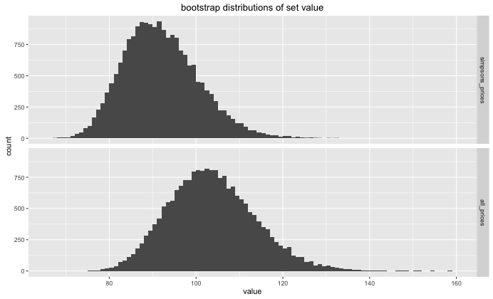
The complete simpsons set seems to average about 96 dollars for a full set, the which is lower than the average for all minifigures $110. This is probably due to the simpsons set being more recent and therefore less rare.
One might wonder though, given these numbers, can we earn a margin by investing in lego minifigures? You can try to tackle this problem with math, but I prefer sampling to keep things simple. Distributed sampling FTW!
cores <- detectCores() # 8 cores on my machine
k <- 16
new_row <- function(n){
  s <- 3000
  p <- 1:s %>%
    map_dbl(~sample(1:k, n, replace = TRUE) %>% unique %>% length) %>%
    map_dbl(~. == 16) %>%
    sum
  c <- 1:s %>%
    map_dbl(~sample(1:k, n, replace = TRUE) %>%
              factor(levels=as.character(1:16)) %>%
              table %>% min) %>%
    mean
  data.frame(n = n, p = p/s, c = c)
}

res <- mclapply(1:800, new_row, mc.cores = cores)

df <- res %>% reduce(rbind)
I can now plot the estimated probability of getting a set after 'n' figures as well as the expected number of sets.
ggplot(data=df %>% filter(n < 100)) +
  geom_point(aes(n, c)) +
  geom_line(aes(n, p)) +
  ggtitle('estimated likelihoods after buying "n" packets')
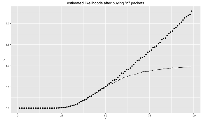
The profit that we can make depends on what price we can sell our excess minifigures for. If we can sell them for 2 dollars (instead of the original 3 dollars) then we are definately in the money if we buy in bulk.
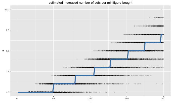
By creating a slightly different visualisation, we can see that the number of minifigures needed to get a new set gets shorter the more minifigures we have.
df <- df %>%
  mutate(sets = round(c))

samplr <- data.frame(
  n = runif(10000, 16, 200) %>% round
) %>%
  mutate(s = n %>% map_dbl(~sample(1:k, ., replace = TRUE) %>%
              factor(levels=as.character(1:16)) %>%
              table %>% min)
)

ggplot() +
  geom_point(data=samplr, aes(n, s), alpha = 0.1) +
  geom_line(data=df %>% filter(n < 200), aes(n, sets),
  color = 'steelblue', size = 2)
Problem with interesting side effects
Suppose that this is an investment opportunity. An interesting property of this investment problem is that the profit from investment increases with the size of the investment. It becomes easier to see if we numerically differentiate the expected number of sets over the number of figures bought.
ma <- function(arr, n=15){
  res = arr
  for(i in n:length(arr)){
    res[i] = mean(arr[(i-n):i])
  }
  res
}

df <- df %>%
  mutate(diff = c - lag(c)) %>%
  filter(!is.na(diff), diff > -1) %>%
  mutate(ma1 = ma(diff), ma2 = ma(ma1), ma3 = ma(ma2))

ggplot() +
  geom_point(data=df, aes(n, diff)) +
  geom_line(data=df, aes(n, ma1))

ggplot() +
  geom_line(data=df, aes(n, ma3)) +
  ggtitle("estimated increased number of sets per minifigure bought, more smoothing")
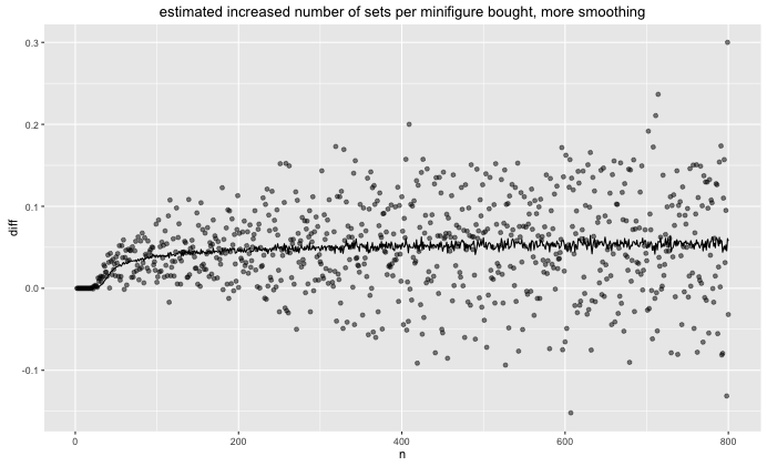
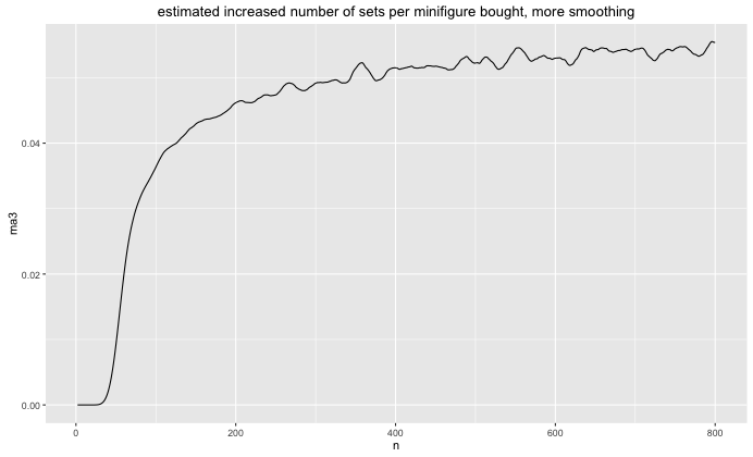
It hasn't completelty seemed to converge. I suppose it might make sense that if you do this until infinity that the convergence would be 1/16 because in the limit you expect to have so many minifigures as a spare that it converges to getting a full set every 16 items you buy (assuming that the likelihood of every figure is equal).
Conclusion
Stochastics like this are very interesting. When you are trying to get your first set, it is hard to get the 16th figure. Once you have your first set, it becomes easier because you've probably got some minifigures left from the last set. This effect stacks. In fact it stacks sofar that you get an unfair advantage over people who have a limited budget. This might explain the suplus on ebay.
I may just invest in lego's this year.