In this document I will illustrate that how a logistic regression can hold up against a support vector machine in a situation where you would expect a support vector machine to perform better. Typically logistic regression fails due to the XOR phenomenon that can occur in data, but there is a trick around it.

The goal of this document is to convince you that you may need to worry more about the features that go into a model, less about which model to pick and how to tune it.

Dependencies

For this experiment I will use python and I'll assume that the following libraries are loaded:

import numpy as np 
import pandas as pd
import patsy 
from ggplot import * 
from sklearn.linear_model import LogisticRegression
from sklearn.svm import SVC
from sklearn.metrics import confusion_matrix

Generate demo data

da = np.random.multivariate_normal([1,1], [[1, 0.7],[0.7, 1]], 300)
dfa = pd.DataFrame({'x1':da[:,0], 'x2': da[:,1], 'type' : 1})
db1 = np.random.multivariate_normal([3,0], [[0.2, 0],[0, 0.2]], 150)
dfb1 = pd.DataFrame({'x1':db1[:,0], 'x2': db1[:,1], 'type' : 0})
db2 = np.random.multivariate_normal([0,3], [[0.2, 0],[0, 0.2]], 150)
dfb2 = pd.DataFrame({'x1':db2[:,0], 'x2': db2[:,1], 'type' : 0})
df = pd.concat([dfa, dfb1, dfb2])

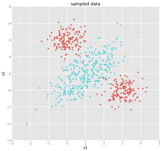
ggplot(aes(x='x1', y='x2', color="type"), data=df) + geom_point() + ggtitle("sampled data")

This should show a dataset similar to this one:

We've generated a classification problem that is impossible to split linearly. Typically we would expect the (linear) logistic regression to perform poorly here and we would expect a (non-linear) support vector machine to perform well.

y,X = patsy.dmatrices("type ~ x1 + x2", df)

Let's see how both models perform now.

Logistic Regression

pred = LogisticRegression().fit(X,ravel(y)).predict(X)
confusion_matrix(y,pred)

Output:

array([[223,  77],
        [118, 182]])

Support Vector Machine

pred = SVC().fit(X,ravel(y)).predict(X)
confusion_matrix(y, pred)

Output:

array([[294,   6],
       [  2, 298]])

The SVM performs much better than the LR. How might we help this?

A dirty trick

Let's see if we can help the logistic regression out a bit. Maybe if we combine x1 and x2 into something nonlinear we may be able capture the problem in this particular dataset better.

df['x1x2'] = df['x1'] * df['x2']
y,X = patsy.dmatrices("type ~ x1 + x2 + x1x2", df)
pred = LogisticRegression().fit(X,ravel(y)).predict(X)
confusion_matrix(y,pred)

Output:

array([[290,  10],
       [  3, 297]])

I am feeding different data to the logistic regression, but by combining x1 and x2 we have suddenly been able to get a non-linear classification out of a linear model. I am still using the same dataset however, which goes to show that being creative with your data features can have more of an effect than you might expect.

Notice that the support vector machine doesn't show considerable improvement when applying the same trick.

pred = SVC().fit(X,ravel(y)).predict(X)
confusion_matrix(y, pred)

Output:

array([[294,   6], 
       [  2, 298]])

Conclusion

Why is this trick so useful?

You can apply a little bit more statistical theory to the regression model which is something a lot of clients (especially those who believe in econometrics) find very comforting. It is less a black box and feels more like a simple regression. Notice that factorization machines are powerfull because they use a very similar approach.

The main lesson here is, before you judge a method useless, it might be better to worry about not putting useless data in it.