A lot of optimisation is done with gradient systems. In this blogpost I’d just like to point out a very simple example to demonstrate that you need to be careful with calling this “optimisation”. Especially when you have a system with a constaint. I’ll pick an example from wikipedia.

Note that you can play with the notebook I used for this here.

The Problem

\[ \begin{align} \text{max } f(x,y) &= x^2 y \\ \text{subject to } g(x,y) & = x^2 + y^2 - 3 = 0 \end{align} \]

This system is a system that has a constraint which makes it somewhat hard to optimise. If we were to draw a picture of the general problem, we might notice that only a certain set of points is of interest to us.

We might be able to use a little bit of mathematics to help us out. We can write our original problem into another one;

\[ L(x, y, \lambda) = f(x,y) - \lambda g(x,y) \]

One interpretation of this new function is that the parameter \(\lambda\) can be seen as a punishment for not having a feasible allocation. Note that even if \(\lambda\) is big, if \(g(x,y) = 0\) then it will not cause any form of punishment. This might remind you of a regulariser. Let’s go and differentiate \(L\) with regards to \(x, y, \lambda\).

\[ \begin{align} \frac{\delta L}{\delta x} &= \Delta_x f(x,y) - \Delta_x \lambda g(x,y) = 2xy - \lambda 2x \\ \frac{\delta L}{\delta y} &= \Delta_y f(x,y) - \Delta_y \lambda g(x,y) = x^2 - \lambda 2 y\\ \frac{\delta L}{\delta \lambda} &= g(x,y) = x^2 - y^2 - 3 \end{align} \] All three of these expressions need to be equal to zero. In the case of \(\frac{\delta L}{\delta \lambda}\) that’s great because this will allow us to guarantee that our problem is indeed feasible! So what one might consider doing is to rewrite this into an expression such that a gradient method will minimise this.

\[q(x, y, \lambda) = \sqrt{\Big( \frac{\delta L}{\delta x}\Big)^2 + \Big( \frac{\delta L}{\delta y}\Big)^2 + \Big( \frac{\delta L}{\delta \lambda}\Big)^2}\]

AutoGrad

It’d be great if we didn’t need to do all of this via maths. As lucky would have it; python has great support for autodifferentiation so we’ll use that to look for a solution. The code is shown below.


from autograd import grad
from autograd import elementwise_grad as egrad
import autograd.numpy as np
import matplotlib.pylab as plt

def f(weights):
  x, y, l = weights[0], weights[1], weights[2]
  return y * x**2

def g(weights):
  x, y, l = weights[0], weights[1], weights[2]
  return l*(x**2 + y**2 - 3)

def q(weights):
  dx = grad(f)(weights)[0] + grad(g)(weights)[0]
  dy = grad(f)(weights)[1] + grad(g)(weights)[1]
  dl = grad(f)(weights)[2] + grad(g)(weights)[2]
  return np.sqrt(dx**2 + dy**2 + dl**2)

n = 100
wts = np.array(np.random.normal(0, 1, (3, )))
for i in range(n):
  wts -= egrad(q)(wts) * 0.01

This script was ran and logged and produced the following plot:

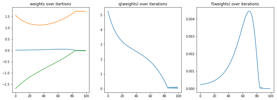
When we ignore the small numerical inaccuracy we can confirm that our solution seems feasible enough since \(q(x, y, \lambda) \approx 0\). That said, this solution feels a bit strange.Taking the found values \(f(x^*,y^*) \approx f(0.000, 1.739)\) suggests that the best value found is \(\approx 0\). Are we sure we’re in the right spot?

The Issue

We’ve used our tool AutoGrad the right way but there’s another issue: the gradient might get stuck in a place that is not optimal. There are more than 1 point that satisy the three derivates shown earlier. To demonstrate this, let us use sympy instead.


import sympy as sp 

x, y, l = sp.symbols("x, y, l")

f = y*x**2
g = x**2 + y**2 - 3 
lagrange = f - l * g

sp.solve([sp.diff(lagrange, x), 
          sp.diff(lagrange, y), 
          sp.diff(lagrange, l)], [x, y, l])

This yields the following set of solutions:

\[\left[\left(0, -\sqrt{3}, 0\right ), \left ( 0, \sqrt{3}, 0\right ), \left ( - \sqrt{2}, -1, -1\right ), \left ( - \sqrt{2}, 1, 1\right ), \left ( \sqrt{2}, -1, -1\right ), \left ( \sqrt{2}, 1, 1\right )\right ]\]

Note that one of these solutions found with sympy yields \((0, \sqrt{3}, 0)\) which corresponds \(\approx [-0.0001, 1.739, -0.0001]\). We can confirm that our gradient solver found a solution that was feasible but it did not find one that is optimal.

A solutions out of our gradient solver can be a saddle point, local minimum or local maximum but the gradient solver has no way of figuring out which one of these is the global optimum (which in this problem is \(x,y = \pm (-\sqrt{2}, 1)\)).

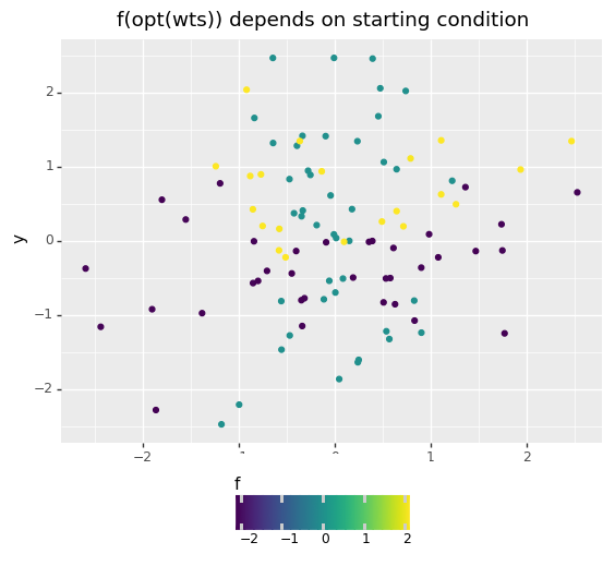
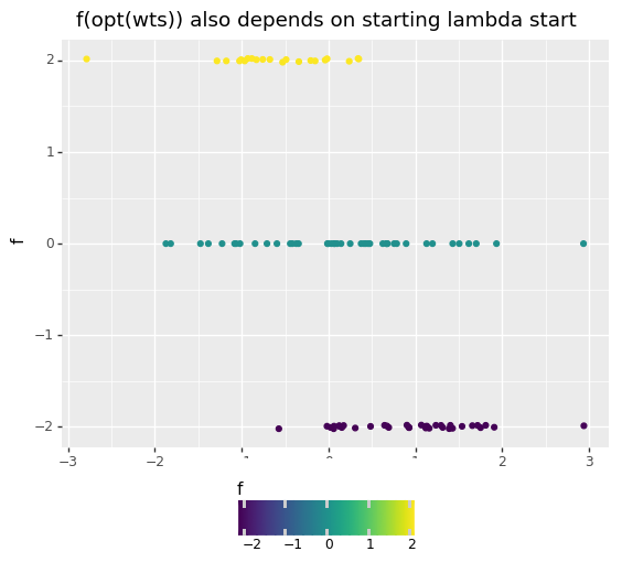
Weather or not we get close to the correct optima depends on the starting values of the variables too. To demonstrate this I’ve attempted to run the above script multiple times with random starting values to see if a pattern emerges.

Some Learnings

This example helps point out some downsides of the gradient approach:

Gradient descent can get stuck in a local (suboptimal) position. The more local optima that exist the trickier it gets to guarantee any form of optimality.
Gradient descent is not really meant to handle constraints. We’ve used a bit of a hack in order to incorporate the constraint into our criterion but it feels more like we’re regularising for it than that we’re using it as a strict constraint.
By adding a constraint to our search we might very well be increaseing the number of local optima that the gradient search might encounter.

In short: gradient descent is a general tactic but when we add a constraint we’re in trouble. It also seems like variants of gradient descent like Adam will also suffer from these downsides.

Why Care?

You might wonder why to care. Many machine learning algorithms don’t have a constraint. Imagine we have a function \(f(x|w) \approx y\) where \(f\) is a machine learning algorithm. A lot of these algorithms involve minimising a system like below;

\[ \text{min } q(w) = \sum_i \text{loss}(f(x_i|w) - y_i) \]

This common system does not have a constraint. But would it not be much more interesting to optimise another type of system?

\[ \begin{align} \text{min } q(w) & = \sum_i \text{loss}(f(x_i|w) - y_i) \\ \text{subject to } h(w) & = \text{max}\{\text{loss}(f(x_i|w) - y_i) \} = \sigma \end{align} \] This would be fundamentally different than regularising the model to prevent a form of overfitting. Instead of revalue-ing an allocation of \(w\) we’d like to restrict an algorithm from ever doing something we don’t want it to do. The goal is not to optimise for two things at the same time but instead we would impose a hard constraint on the ML system.

Another idea for an interesting constraint:

\[ \begin{align} \text{min } q(w) & = \sum_i \text{loss}(f(x_i|w) - y_i) \\ \text{subject to } & \\ h_1(w) & = \text{loss}(f(x_1|w) - y_1) \leq \epsilon_1 \\ & \vdots \\ h_k(w) & = \text{loss}(f(x_k|w) - y_k) \leq \epsilon_k \end{align} \] The idea here is that one determines some constraints \(1 ... k\) on the loss of some subset of points in the original dataset. The idea here being that you might say “these points must be predicted within a certain accuracy while the other points matter less”.

\[ \begin{align} \text{min } q(w) & = \sum_i \text{loss}(f(x_i|w) - y_i) \\ \text{subject to } & \\ h_1(w) & =\frac{\delta f(x|w)}{\delta x_{k}} \geq 0 \\ h_2(w) & =\frac{\delta f(x|w)}{\delta x_{m}} \leq 0 \end{align} \] Here we’re trying to tell the model that for some feature \(k\) we demand a monotonic increasing relationship with the output of the model and for some feature \(m\) we demand a monotonic decreasing relationship with the output. For some features a modeller might be able to declare upfront that certain features should have a relationship with the final model and being able to constrain a model to keep this in mind might make the model a lot more robust to certain types of overfitting.

Dreams

This flexibility of modelling with constraints might do wonders for interpretability and feasibility of models in production. The big downer is that currently we do not have general tools to guarantee optimality under constraints in general machine learning algorithms.

That is, this is my current understanding. If I’m missing out on something: hit me up on twitter.

\(\text{hack} \neq \text{fix}\)

As a note I figured it might be nice to mention a hack I tried to improve the performance of the gradient algorithm.

The second derivatives of \(L\) with regards to \(x,y\) also need to be negative if we want \(L\) to be a maximum. Keeping this in mind we might add more information to our function \(q\).

\[q(x, y, \lambda) = \sqrt{\Big( \frac{\delta L}{\delta x}\Big)^2 + \Big( \frac{\delta L}{\delta y}\Big)^2 + \Big( \frac{\delta L}{\delta \lambda}\Big)^2 + \text{relu} \Big(\frac{\delta L}{(\delta x)^2}\Big)^2 + \text{relu} \Big(\frac{\delta L}{(\delta y)^2}\Big)^2}\]

The reason why I’m adding a \(\text{relu}()\) function here is because if the second derivative is indeed negative the error out of \(\text{relu}()\) is zero. I’m squaring the \(\text{relu}()\) effect such that the error made is in proportion to the rest. This approach also has a big downside though: the relu has large regions where the gradient is zero. So we might approximate with a softplus instead.

\[q(x, y, \lambda) = \sqrt{\Big( \frac{\delta L}{\delta x}\Big)^2 + \Big( \frac{\delta L}{\delta y}\Big)^2 + \Big( \frac{\delta L}{\delta \lambda}\Big)^2 + \text{softplus} \Big(\frac{\delta L}{(\delta x)^2}\Big)^2 + \text{softplus} \Big(\frac{\delta L}{(\delta y)^2}\Big)^2}\]

I was wondering if by adding this, one might improve the odds of finding the optimal value. The results speak for themselves:

with softplus 310/1000 solutions hit the proper value
without 300/1000 solutions hit the proper value

Luck might be a better tactic.