In this document I'll explore an optimal stopping problem that occurs in popular dungeons and dragons games. It features probability theory and the python itertools package.
Screenshot
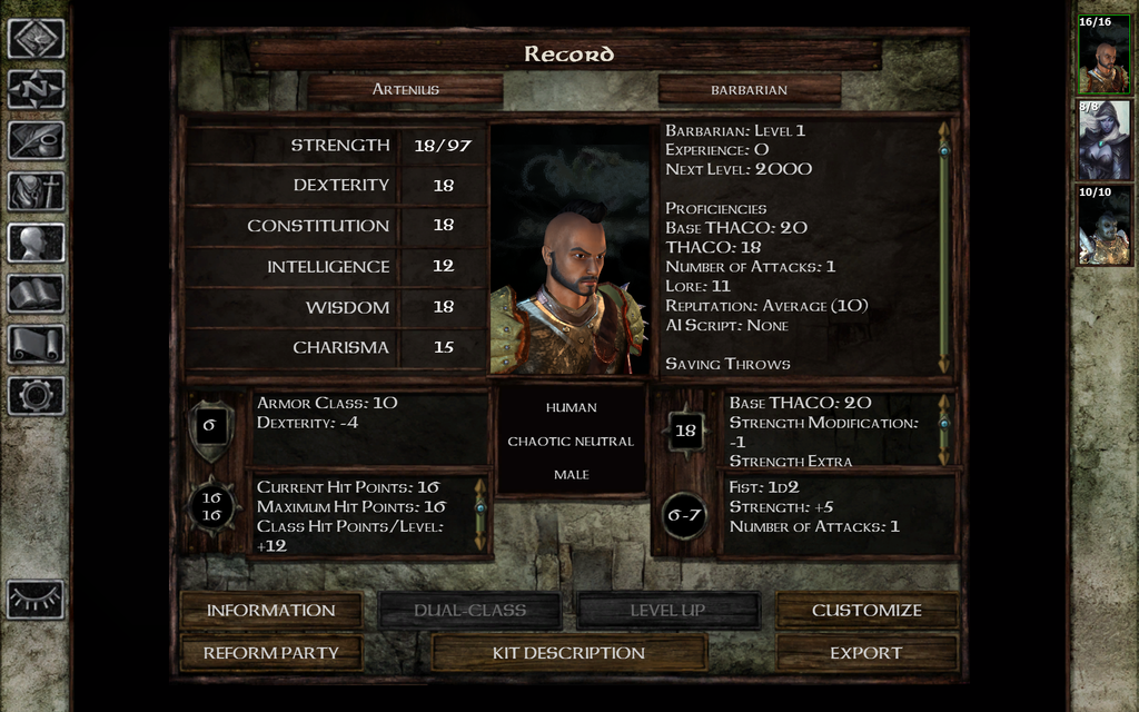
This is a screenshot of a video game I used to play when I was 12. This is the character screen and you can see the attributes of the hero. Depending on the class of the hero you typically value certain attributes over others. This screenshot shows a lot of value in strength and constitution so it is probably a brawler of some sort instead of a wizard who prefers intelligence.
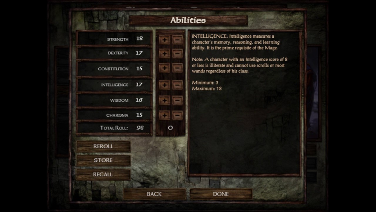
When you create a character in this video game, which is based off of dungeons and dragons, you need to roll dice which determine how many points in total you can allocate to your character. There is no penalty for rerolling besides the time that you've wasted rerolling. I couldn't be too bother back when I was twelve but there are people who celebrate a high roll with videos on youtube and there are forums with plenty of discussions.
Stochastics
There's something stochastic which is interesting about this dice rolling problem. You want to have a high score but you don't want to end up rerolling a lot. So what is a good strategy?
This got me googling, again, for a fan website which had the rules for character generation. It seems that the system that generates scores is defined via three rules.
1. Roll 4 six sided dice, remove the lowest die. Do this 6 times (for each stat).
2. If none of the stats are higher than a 13, start over at step 1.
3. If the total modifiers are 0 or less, start over at step 1
(I belive this translates to the score needing to be greater than 60 ).
Let's turn this system into a game. You are allowed to reroll, but everytime you do the score you get will get subtracted by one. What would be the optimal stopping strategy?
We need to infer some probabilities first and there's two methods of getting them.
Approach 1: Simulation
It feels like we may need to consider $(6^4)^6$ different combinations that are possible so we could avoid enumeration via simulation. The following code will give us approximate probabilities that should work reasonably well.
import random
from collections import Counter

def roll_attr():
    rolls = [random.randint(1,6) for _ in range(4)]
    return sum(sorted(rolls)[1:])

def simulate_char():
    stat = [0,0,0,0,0,0]
    bad_char = True
    while bad_char:
        stat = [roll_attr() for _ in stat]
        bad_char = (max(stat) <= 13) or (sum(stat) < 60)
    return stat

n = 10000
c = Counter([sum(simulate_char()) for _ in range(n)])
probs = {k:v/n for k,v in dict(c).items()}

def p_higher(val):
    return sum([v for k,v in probs.items() if k >= val])
Approach 2: Enumeration
Give it some thought and you may actually be able to iterate through all this. It won't be effortless but you could go there.
You may wonder how though. After all we need to roll 4 normal dice for every attribute and we need to do this for each of the six attributes. This sounds like you need to evaluated $(6^4)^6$ possible dice outcomes. Sure you may be able to filter some of the results away, but it is still a scary upper limit. Right?
To show why this is pessimistic, let's first consider all the dice combinations for a single attribute. We could enumerate them via;
import itertools as it

d = (1,2,3,4,5,6)
roll_counter = Counter((_ for _ in it.product(d,d,d,d)))
This roll_counter object now contains all the possible rolls and counts them. In total it has the expected $6^4=1296$ different tuples. We don't want to consider all these possible rolls though. We will throw away the lowest scoring roll. Let's accomodate for that.
roll_counter = Counter((tuple(sorted(_)[1:]) for _ in it.product(d,d,d,d)))
This small change causes our roll_counter object to only have 56 keys. The upper limit of what we need to evaluate then is $56^6 = 30.840.979.456$. That's a lot better. We can reduce our key even further though.
roll_counter = Counter((sum(sorted(_)[1:]) for _ in it.product(d,d,d,d)))
This object only has 16 keys. Why can we do this? It's because we are not interested in individual dice rolls but we're interested in the scores that are rolled per attribute. By counting the scores we still keep track of the likelihood of each score without having to remember all of the dice rolls. This brings us to $16^6=16.777.216$ we may need to evaluate which is a number we can deal with on a single machine. We will even filter some of the rolls away because we need to reroll when the total scores are less than 60.
How many total objects do we need to consider?
k = roll_counter.items()

def roll_gt(tups, n):
    min([_[0] for _ in tups]) > 13
    return sum([_[0] for _ in tups]) > 60

sum(1 for comb in it.product(k,k,k,k,k,k) if roll_gt(comb, 60))
Turns out we only need to iterate over 9.822.736 items because many of the rolls are infeasible.
This should be doable, but let's be careful that we apply maths correctly.
def map_vals(tups):
    rolled_value = sum([_[0] for _ in tups])
    how_often = reduce(lambda x,y:x*y, [_[1] for _ in tups])
    return Counter({rolled_value: how_often})
%time folded = reduce(op.add, it.islice(mapped, 100000))
CPU times: user 4min 58s, sys: 1.38 s, total: 5min
Wall time: 5min 1s
Not bad!
Comparison
At this stage it is not a bad idea to check if I've not made a mathematical error. Let's compare the two plots.
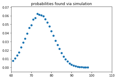
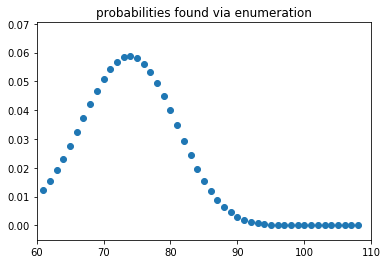
Nothing jumps out as extraordinary so I think I'm good. I'll use the enumerated probabilities for all steps to come.
Toward Decision Theory
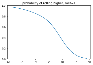
We need to calculate the probability that you'll get a higher score if you roll again.
The goal is not to get a higher score in this one next roll, but a higher score in any roll that comes after. Intuitively this probability is defined via;
$$ \begin{split} \mathbb{P}(\text{higher than } s_0 \text{at roll } r) = & \mathbb{P}(s_1 > s_0 + r + 1) + \\ & \mathbb{P}(s_2 > s_0 + r + 2)\mathbb{P}(s_1 \leq s_0 + r + 1) + \\ & \mathbb{P}(s_3 > s_0 + r + 3)\mathbb{P}(s_2 \leq s_1 + r + 1)\mathbb{P}(s_1 \leq s_0 + r + 1) + \\ & \mathbb{P}(s_4 > s_0 + r + 4)\mathbb{P}(s_3 \leq s_2 + r + 1)\mathbb{P}(s_2 \leq s_1 + r + 1)\mathbb{P}(s_1 \leq s_0 + r + 1) + \\ & ... \end{split} $$
We need to abstract this away into some python code. But it is not too hard. I'll use numba.jit to make some parts a bit quicker though.
import numba as nb

def p_higher_next(val, probs):
    return sum([v for k,v in probs.items() if k >= val])


def prob_higher(score, n_rolls, probs):
    if score <= 60:
        raise ValueError("score must be > 60")
    p = 0
    for roll in range(n_rolls + 1, max(probs.keys())+1):
        higher_p = p_higher_next(score + roll, probs)
        fails_p = reduce(lambda a,b: a*b, [1] + [1-p_higher_next(score + _, probs) for _ in range(roll - n_rolls - 1)])
        p += higher_p*fails_p
    return p


@nb.jit
def decisions_matrix(probs, choice=lambda x: x):
    matrix = []
    for score in reversed(list(probs.keys())):
        row = []
        for roll in range(1,25):
            output = prob_higher(score, roll, probs)
            output = choice(output)
            row.append(output)
        matrix.append(row)
    return matrix

def plot_decisions(probs, choice=lambda x: x, title=""):
    mat = decisions_matrix(probs, choice)
    plt.imshow(mat,
               interpolation='none',
               extent=[1, len(mat_p[0]), min(probs.keys()), max(probs.keys())])
    plt.title(title)
    _ = plt.colorbar();
All this code will generate the probabilities we want and we can visualise the results.
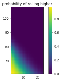
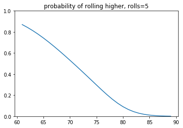
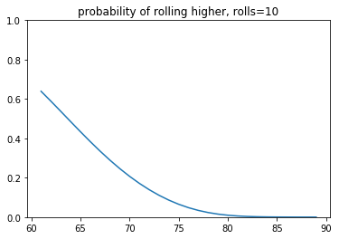
- The first plot demonstrates the probability of getting a higher score given a current score and the number of rolls you currently have.
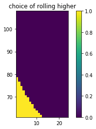
- The second plot rounds these probabilities, giving us a decision boundary.
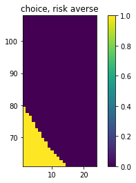
- The third plot rounds these probabilities but assumes we are less risk averse. We add 0.1 mass to each probability.
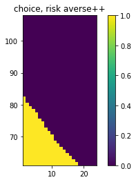
- The third plot does the same but even more risk seeking. We add 0.3 mass to each probability.
You may notice that it seems like adding more probability mass doesn't change the behavior much. This is partly due to the visual bias in the y-axis (the odds of ever getting a score >90 are slim indeed). Another reason is that the switchpoint of the decision making region is very steep. So you'd need to really bias the risk if you want to see a change in decision making. These plots might shed some light on that phenomenon.
At this point, I was content with my work but then I had a discussion with a student who suggested a much simpler tactic.
Making the model too simple
The student suggest that the solution could be much simpler. Namely we merely needed to optimise;
$$ \text{argmax } v(a| s, t)= \begin{cases} s - t,& \text{if } a\\ \mathbb{E}(s) - t - 1 & \text{if not } a \end{cases} $$
Where $s$ is the current score, $t$ is the number of turns we've currently rerolled and $a$ denotes the action of stopping.
This suggests optimising a linear system based on expected value. To demonstrate that this is wrong, let's first calculate the expected value.
> sum([k*v for k,v in probs_iter.items()])
74.03527564970476
Let's now compare how this decision rule compares to our previous decision rule. The linear tactic is shown with a red line.
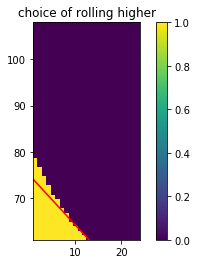
The naive model seems to fail to recognize that early on, re-rolling is usually a good tactic. The linear model only compares to getting a higher probability in the next reroll, not all rerolls that will happen in the future. If the student would have picked to optimise the following, it would have been fine;
$$ \text{argmax } v(a| s, t)= \begin{cases} s - t,& \text{if } a\\ \mathbb{E}(s, t) - 1 & \text{if not } a \end{cases} $$
It can be easy to make mistakes while optimising the correct model, but the easiest mistake is to pick the wrong model to start with.
Conclusions
I like this result and I hope it serves as a fun example on decision theory. I've made some assumptions on the D&D rules though because I didn't feel like reading all of the rules involved with rolling. It is safe to assume that my model is flawed by definition.
This "icewind dale problem" is very similar to the "secretary problem" or the "dating problem". All these problem focus on finding the right moment to stop and reap the benefits. The problems differ on a few things which can make the problem harder:
- in our problem we are always able to reroll, you could imagine a situation where there is a chance of being able to reroll
- we knew the stochastic process that generates scores beforehand, you could imagine that if we do not know how the attribute scores are generated that the problem becomes a whole lot harder too
Then looking back at how I solved this problem I'd like to mention a few observations too.
- This is a rare case where you are able to enumerate the probabilities instead of simulating them. I find that you should celebrate these moments by doing the actual work to get the actual probabilities out. It requires more mental capacity though, initially working with simulations may also just be fine if you're just exploring.
- I took the proper math path and I showed that the $\text{argmax } \mathbb{E}(s)$ expected value heuristic is flawed, albeit not too far off. If you only want to spend 5 minutes on the problem I guess simulation simulation and the expected value heuristic heuristic should get you 80% of the way for 5% of the time though.
- You don't always need numeric libraries like
numpy. What makes python great for these sorts of things is that I did not need to make custom objects because I was able to make use of the great little libraries in the standardlib. Tools likefunctools.reduce,collections.Counteranditertoolsreally make solving these problems fun.
From here there are many other cool things you could calculate though. Given that you want at least a score of 88, how long do you expect to be rolling? If you feel like continueing my work, feel free to grab the notebook I used here.