I've gotten a bit bothered lately with some practices in ML. Students that get out of college seem to learn a lot about deeper and complexer models at the cost of proper methodology. In this blogpost I hope to demonstrate how this way of thinking about models can be incredibly naive.

Enter Chickweight

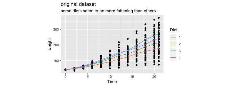
Let's consider my favorite dataset: chickweight. It is a dataset that comes with R and it depicts chickens that each receive one of four diets. The goal of the dataset is to figure out what the effect is of the diet on the chickens growth. The first few rows look like this:

  weight time chick diet
1     42    0     1    1
2     51    2     1    1
3     59    4     1    1
4     64    6     1    1
5     76    8     1    1
6     93   10     1    1

The plot that summarises it best is shown below.

Let's now make some models on this dataset. I'll try three approaches and we will see that they are all wrong. By demonstrating why they are wrong we can come to another method of modelling that might give use a correct model.

Approach 1: simple linear regression

Let's do standard one-hot-encoding and a simple linear model.

model <- lm(weight ~ Time + Diet, data=chickweight)

To explain what I don't like about this model I'll compare the original chart with the one below.

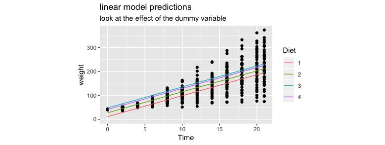
A few things that I do not like.

the intercept is different for each diet
the slope is the same for each diet
it should be the other way around

Approach 2: feature engineering

To try and adress some of these issues I'll apply some R voodoo magic such that I can train a different model for each diet. So ever diet will have it's own slope and it's own intercept. In R it is actually suprisingly easy to code this up.

pltr <- chickweight %>%
  group_by(Diet) %>%
  nest() %>%
  mutate(mod = data %>% map(~ lm(weight ~ Time, data=.)),
         pred = data %>% map2(mod, ~ predict(.y, data=.x))) %>% 
  unnest(data, pred)

Below is a plot of the predictions.

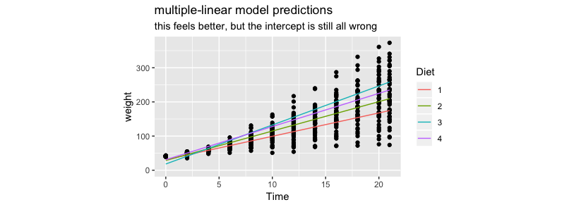
This approach feels better but I'm again a bit disturbed by the fact that the intercepts are all different.

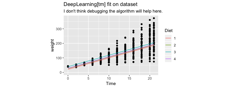
Approach 3: DeepLearning[tm]

Maybe I should try and see if DeepLearning[tm] can help me.

model <- keras_model_sequential() 
model %>% 
  layer_dense(units = 6, activation = 'relu', input_shape = c(5)) %>% 
  layer_dropout(rate = 0.2) %>% 
  layer_dense(units = 4, activation = 'relu') %>%
  layer_dropout(rate = 0.1) %>%
  layer_dense(units = 1, activation = 'linear')

Nope, same issues.

Actual Modelling

The previous approaches didn't really work for me.

Instead of trying out machine learning approaches where we cram our data into a predefined machine learning model: let's do something different. How about we actually try to model the problem! We'll no longer push our dataset into a predefined model. Instead we'll just grab a bit of pen and paper and write down what we want the model to actually do.

Here's what I first came up with.

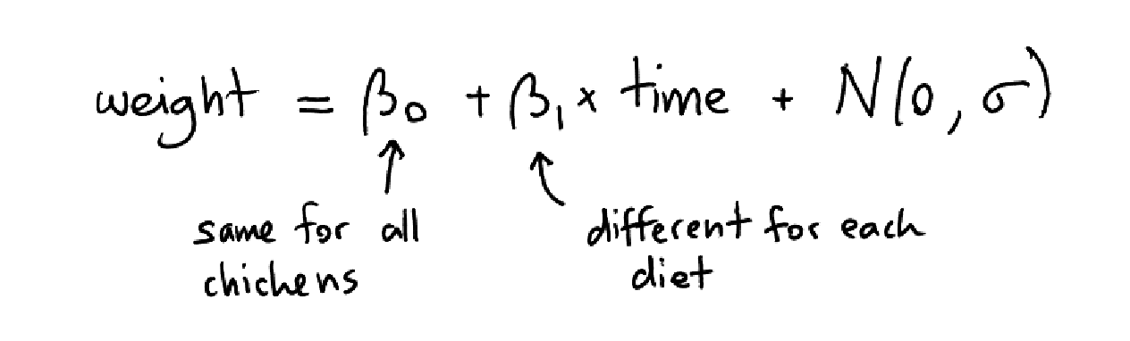
I want to make a simple linear model where the intercept is the same for all chickens and where the slope is only dependant on the diet of the chicken. You might still be able to get here with a simple linear model and some clever feature engineering. In the long run this won't work though because we might want to make some further iterations. Instead of hoping for a proper mold to fit the data in it might make sense to implement this in a probibalistic programming tool instead.

It's easier than you might think. Here's an implementation in R.

library(rethinking)
mod <- map2stan(alist(
    weight ~ dnorm(mu, sigma),
    mu <- intercept + slope[Diet]*Time,
    slope[Diet] ~ dnorm(0, 2),
    intercept ~ dnorm(0, 2),
    sigma ~ dunif(0, 10)
  ), iter = 5000, data = chickweight, warmup = 500)

Not only is this a flexible programming exerperience but you also get uncertainty bounds for using a bayesian tool as well.

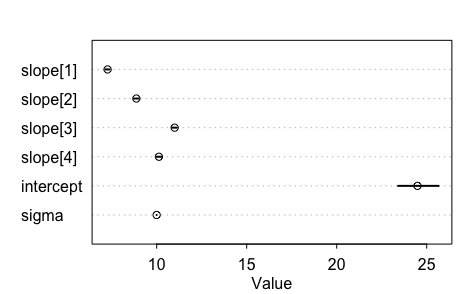
Apon inspecting the results I noticed that something bad was happening. The intercept isn't at all where I expected it to be. Let's look at our initial plot one more time.

The intercept should be around 40-ish. I also seem to have forgotten to model the variance increasing over time. After considering this, I went back to my model on the drawing board and wrote some extra specifications.

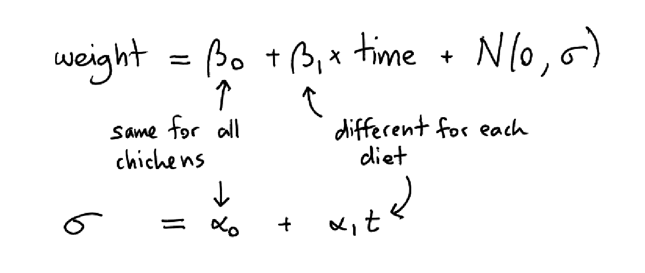
The luxury of a probibalistic programming tool is that I can just add variables and have the model run. I am not limited by the models in my toolbox, I can just write my own using whatever domain knowledge I have.

mod <- map2stan(
 alist(
   weight ~ dnorm(mu, sigma),
   mu <- beta_0 + beta_1[Diet]*Time,
   beta_0 ~ dnorm(0, 2),
   beta_1[Diet] ~ dnorm(0, 2),
   sigma <- alpha_0 + alpha_1[Diet]*Time,
   alpha_0 ~ dunif(0, 10),
   alpha_1[Diet] ~ dunif(0, 10)
 ), data = chickweight, warmup = 500)

The results from this now look a lot better.

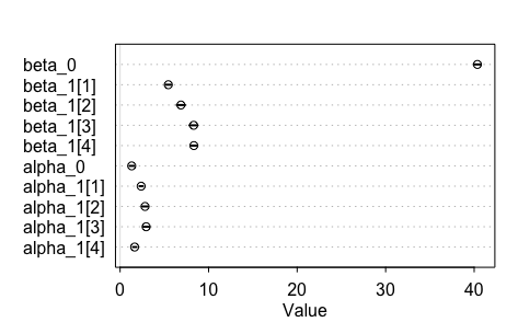
That reinterpretation of sigma meant a whole lot of difference! Glad that I've got a tool that allows me to model it this way.

Statistical Bonus

There's something extra precious happening here. Suppose now that I wanted to say which diet is best for getting the chickens fat. If I wanted to do a statistical test on the chickens at the latter timesteps of the dataset then I wouldn't have enough data. This dataset is "small data".

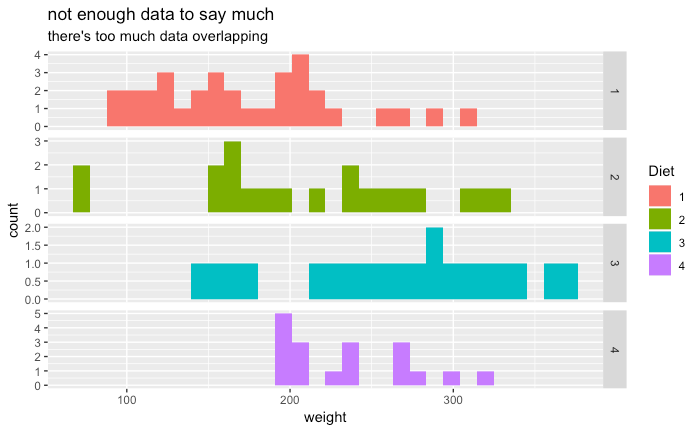
But when we instead look at the average growth for every chicken for every timestep then we suddenly do seem to have enough data to make a few statistical statements. Let's look at that final chart one more time.

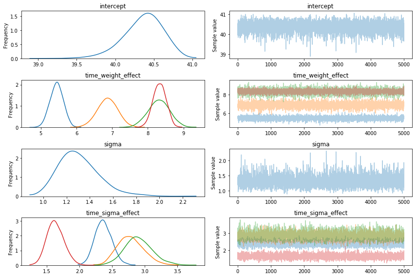
What we're looking at are posteriors that have been fitted to the data. The graphic suggests to us that diet 3 and 4 (look at the values for beta_1) give us statistically heavier chickens. Note that it also shows us that the variance for diet 4 is the more statistically stable of the two (look at the values for alpha_1).

Having a model with this articulate property is amazing, note:

not only could we use this model for prediction, but we can also use it for hypothesis testing
not only do we get a trained model, but also a model with uncertainty bounds built in
we can fully explain the model, which is nice for GDPR reasons

These properties are kind of great when you think about it and they're often missing from other popular algorithms like ensemble methods and deep learning.

PyMC3

This way of modelling isn't reserved for just R. To show it, here's the same model but in PyMC3.

import pandas as pd 
import numpy as np 
import pymc3 as pm
import matplotlib.pylab as plt
%matplotlib inline

df = pd.read_csv("http://koaning.io/theme/data/chickweight.csv", 
                 skiprows=1,
                 names=["r", "weight", "time", "chick", "diet"])

df = df.sample(frac=1.0)
dummy_rows = pd.get_dummies(df.diet)

with pm.Model() as mod: 
    intercept = pm.Normal("intercept", 0, 2)
    time_effect = pm.Normal("time_weight_effect", 0, 2, shape=(4,))
    diet = pm.Categorical("diet", p=[0.25, 0.25, 0.25, 0.25], shape=(4,), observed=dummy_rows)
    sigma = pm.HalfNormal("sigma", 2)
    sigma_time_effect = pm.HalfNormal("time_sigma_effect", 2, shape=(4,))
    weight = pm.Normal("weight", 
                       mu=intercept + time_effect.dot(diet.T)*df.time, 
                       sd=sigma + sigma_time_effect.dot(diet.T)*df.time, 
                       observed=df.weight)
    trace = pm.sample(5000, chains=1)

Note that PyMC3 also gives us a nice traceplot too.

Conclusion

I hope this example demonstrates a clear benefit of manually modelling for the sake of articulate models. I'm not suggesting this is always the best path forward; you can often get far with an sklearn pipeline too but we should acknowledge the benefits of these articulate models:

we can quantify uncertainty in our output
we can describe the model using domain knowledge
we can explain why a certain decision was made

I would like to point out though, that even with this type of modelling lots of things can still go wrong. In this dataset in particular, there are some chickens that seem to have died prematurely! The model would still not be able to tell you this, you'd still need to do the legwork yourself.

koaning.io

Towards Articulate Models