In this document I'll demonstrate that any bayesian algorithm is also an algorithm that can be implemented for streaming. If not for streaming, it also turns out that an alternative benefit is that the algorithm becomes parallel. I'll demonstrate this with a little bit with maths and then with a demo linear regression application in python. I'll conclude by preaching a founding idea of apache flink.

Bayes Rule for Parameters

Bayesian have a different way of thinking about modelling (see a previous blogpost). Whenever a bayesian models they immediately write down the following:

$$ p(\theta | D) \propto p(D | \theta) p (\theta) = \Pi_i p(d_i | \theta) p(\theta) $$

This formula is very important as it gives us another way to make models via inference. In the context of streaming, it even tells us something extra. Let's consider three independant points of data that we've seen; $d1, d2, d3$. Then bayes rule states that;

$$ p(\theta | d_1, d_2, d_3) \propto p(d_3 | \theta) p(d_2 | \theta) p(d_1 | \theta) p(\theta) $$

You may recognize a recursive relationship here. When the 3rd datapoint comes in, it moves probability mass based on the prior knowledge known (based on $d_2, d_1$ and the original prior). When the 2nd datapoint comes in, it moves probability mass based on the prior knowledge know (based on just $d_1$ and the original prior).

$$p(\theta | d_1, d_2, d_3) \propto p(d_3 | \theta) p(d_2 | \theta) \underbrace{p(d_1 | \theta) p(\theta)}_{\text{prior for } d_2} $$

$$p(\theta | d_1, d_2, d_3) \propto p(d_3 | \theta) \underbrace{p(d_2 | \theta) p(d_1 | \theta) p(\theta)}_{\text{prior for } d_3} $$

When a model is written down in this form we gain an interesting property: the model updates after each datapoint comes in. The new model depends only on the previous model and a new datapoint. This means it has one very interesting consequence;

Any ML algorithm that can be written via $ p(\theta | D) \propto \Pi_i p(d_i | \theta) p(\theta)$ is automatically a streaming algorithm as well.

Turns out, lots of algorithms can be turned into streaming algorithms this way. Another nice property shows itself: if each $p(d_i | \theta)$ is independant of eachother then we can also process parts of $\Pi_i p(d_i | \theta)$ in parallel as long as we combine it in the end. Map-Reduce ahoy!

Streaming Regression

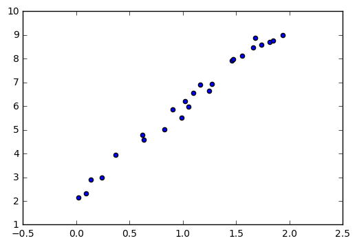
Let's first generate some simple regression data that we need to work with.

import matplotlib.pyplot as plt
import tensorflow as tf
import numpy as np 
import scipy as sp
import pandas as pd 
import numba as nb
%matplotlib inline  

n = 25
xs = np.random.uniform(0, 2, n)
ys = 2.5 + 3.5 * xs + np.random.normal(0, 0.3, n)
plt.scatter(xs, ys)

We will now try to model this dataset. Again, we'll write down what every bayesian does;

$$ p(\theta | D) \propto p(D | \theta) p (\theta) = \Pi_i p(d_i | \theta) p(\theta) $$

To keep things simple, we'll take $\theta = [w_0, w_1]$. That is, I'll not worry about the variance and I am merely interested in figuring out the posterior distribution of the intercept and the slope. I'll assume $p(\theta)$ to be uniform. If we keep things basic like this, I'll only need to worry about the likelihood $p(d_i | \theta)$.

Here's my proposed model:

$$ p(d_i | \theta) \sim N(w_0 + w_1 x - y, \sigma^2) = \frac{1}{\sqrt{2\pi} \sigma} \exp{ \frac{(w_0 + w_1 x - y)^2}{2\sigma^2} } $$

I'll asumme $\sigma = 1$ just to keep the plotting simple and two dimensional. You could go a step further and model $\theta = [w_0, w_1, \sigma]$ but we'll skip that in this document.

With this likelihood known, we can now write code for it. I'll write a function that I'll keep fast by applying numba.

@nb.jit
def likelihood(x, y, n = 101, bmin = -5, bmax = 5):
    res = np.zeros((n,n))
    for i, b0 in enumerate(np.linspace(bmin, bmax, n)):
        for j, b1 in enumerate(np.linspace(bmin, bmax, n)):
            res[n - 1 - j, i] =  np.exp(-(b0 + b1*x - y)**2/2)/np.sqrt(2*np.pi)
    return res/np.sum(res)

Let's demonstrate the likelihood.

plt.figure(figsize=(5,5))
_ = plt.imshow(likelihood(x = 1, y = 2), 
           interpolation='none', extent=[-5, 5, -5, 5])
plt.xlabel('$w_0$')
plt.ylabel('$w_1$')
plt.title('$p(x=1, y=2 | w_0, w_1)$')
_ = plt.colorbar()

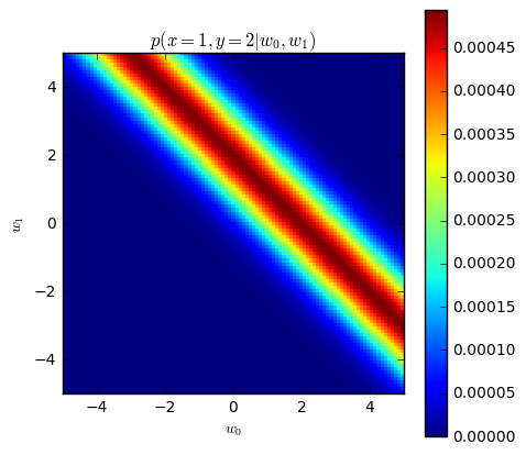
You may be wondering about the shape of this distribution. The shape makes sense when you realize $w_0$ and $w_1$ 'negatively correlated'. Suppose we have a line that goes through the point, then the only way to increase the intercept while still going through the point is to decrease the slope (and vise versa).

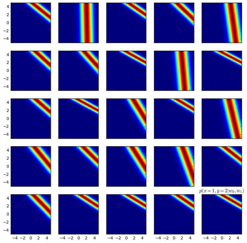
We just showed a likelihood chart for a single point but we can also make this for every point of data in our dataset.

f, axes = plt.subplots(5, 5, sharex='col', sharey='row', figsize = (10, 10))
# flatten the list to make iteration easier 
axes = [item for sublist in axes for item in sublist]

# loop over axes and create the plot 
for dim, axis in enumerate(axes):
    axes[dim].imshow(likelihood(xs[dim], ys[dim]), 
                     interpolation='none', extent=[-5, 5, -5, 5])

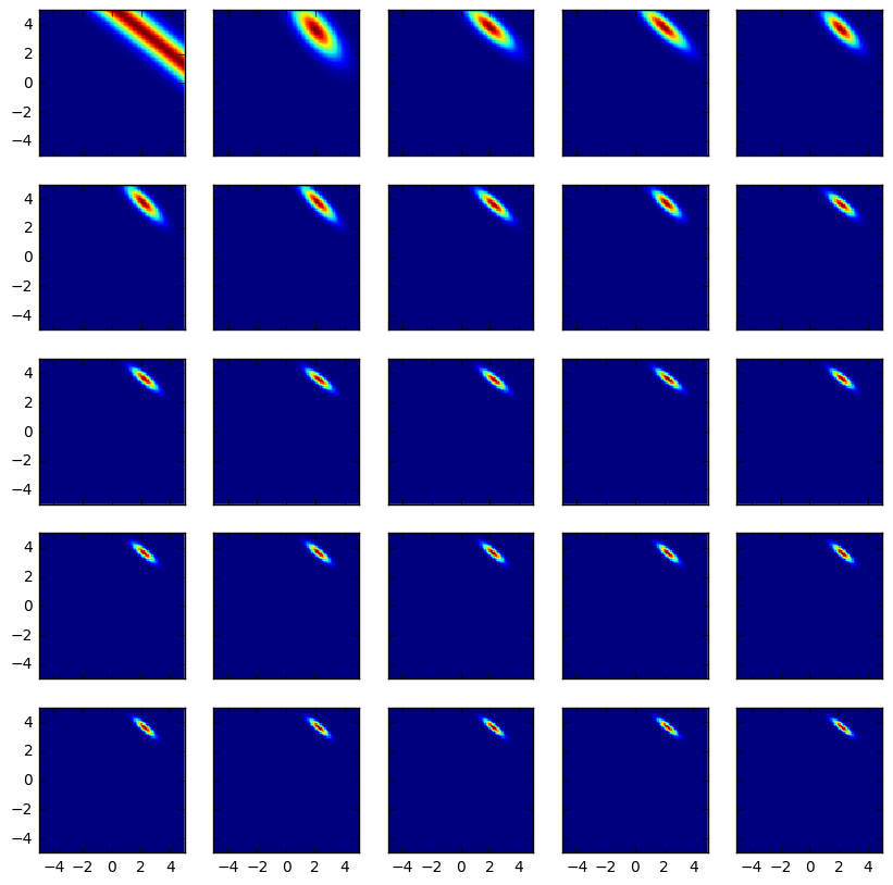
Let's now apply the recursive relationship we mentioned at the beginning of the blogpost. Let $D_N$ be the data seen until now and let $d_{N+1}$ be the new datapoint that is just arriving at the model.

$$p(\theta | D_N, d_{N+1}) \propto p(d_{N+1} | \theta) \underbrace{p(D_N| \theta) p(\theta)}_{\text{prior for new datapoint}} $$

We can show how the posterior distribution changes as we add more and more points. Notice the convergence.

f, axes = plt.subplots(5, 5, sharex='col', sharey='row', figsize = (10, 10))
axes = [item for sublist in axes for item in sublist]

res = []
for dim, axis in enumerate(axes):
    if len(res) != 0:
        res = res * likelihood(xs[dim], ys[dim])
        res = res/np.sum(res)
    else: 
        res = likelihood(xs[dim], ys[dim])
    axes[dim].imshow(res, 
                     interpolation='none', extent=[-5, 5, -5, 5])

Let's zoom in on the final posterior.

plt.figure(figsize=(5,5))
_ = plt.imshow(res, interpolation='none', extent=[-5, 5, -5, 5])
plt.xlabel('$w_0$')
plt.ylabel('$w_1$')
plt.title('$p(w_0, w_1 | D)$')

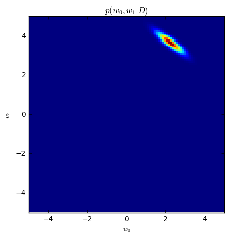
The true values for $w_0, w_1$ are 2.5 and 3.5. From eyeballing at the posterior I'd say this method seems to work.

Extra Modelling Options

Currently we've implemented a streaming model for linear regression that tries to learn static parameters. How would we change this model if these parameters aren't static?

Answer, we can fiddle around with the recursive relationship. Remember;

$$p(\theta | D_N, d_{N+1}) \propto p(d_{N+1} | \theta) p(D_N | \theta)$$

Let's introduce a parameter $\alpha$ that gives more weight to the likelihood distribution of the most recent datapoint. We can combine the idea of exponentially weighted smoothing with our bayesian mindset to get to a model that will give more mass to points that are recent.

$$p(\theta | D_N, d_{N+1}) \propto p(d_{N+1} | \theta) p(D_N | \theta) + \alpha p(d_{N+1} | \theta)$$

We still retain the streaming aspect of the model but we are applying a bit of hack as far as probability theory is concerned.

A thing of beauty

Looking at the problem with bayesian glasses gives benefits over just looking at it from the standard ML/frequentist point of view. The alternate way of thinking has supplied us with a neat probabilistic mindset that allows us to tackle streaming problems with ease.

We could now apply a koan; instead of asking ourselves how to solve streaming problems we may wonder if streaming problems are any different than batch. The observation being; if you've solved streaming then you've also solved batch. After all, we can stream a large file into the algorithm line by line.

Mind blown. If you've solved streaming, you've just solved batch as well.

Exactly this attitude is what makes apache flink such a badass project. Flink offers a framework to do streaming analytics on a distributed system. Spark also has some support for this problem but cheats a little bit by not offering 'true' streaming but by offering microbatching. I expect these two framework to fight for control of the ecosystem in the next year. Not everybody has the same latency requirements.

Another main benefit of being able to do streaming algorithms is that your system will have less moving parts. Most web applications suffer from all the extra work involved with the integration of caching systems, oozie jobs, model serialisation and monitoring. If your model can just learn on a stream, all this would be done in one go.

Conclusion

Batch is a subset of streaming and thinking like a bayesian helps when designing models.