In a previous document I described how bayesian models can recursively update, thus making them ideal as a starting point for designing streaming machine learning models. In this document I will describe a different method proposed by Crammer et al. which includes a passive agressive approach to model updates. I will focus on intuition first before moving to the mathy bits. At the end I will demo some sklearn code with implementations of these models.
Intuition
Step 1
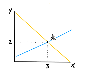
Let's say you're doing a regression for a single data point $d_i$. If you only have one datapoint then you don't know what line is best. The yellow line will pass through the point perfectly and so will the blue line.
Step 2
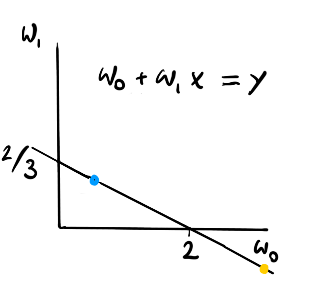
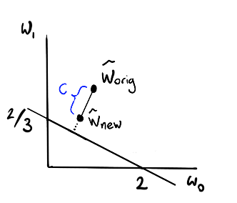
We can describe all the lines that will go through the line perfectly though. If we make a plot of the weight space of the linear regression ($w_0$ is the constant and $w_1$ is the slope) we can describe all the possible perfect fits with a line.
Note that the blue dot corresponds to the blue line and the yellow point corresponds to the yellow line.
Step 3
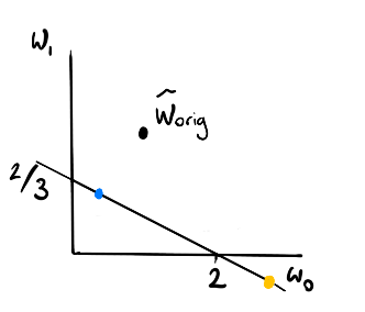
Any point on that line is as good as far as $d_i$ is conserned so which point has the most value?
How about we compare it to the weights that the regression had before it came across this one point? Let's call these weights $w_{\text{orig}}$.
In that case the blue regression seems better than the yellow one but is it the best choice?
Step 4
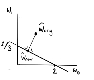
This is where we can use maths to find the coordinate on the line that is as close as our original weights $w_{\text{orig}}$.
In a very linear system you can get away with linear algebra but depending on what you are trying to do you may need to introduce more and more maths to keep the update rule consistent.
Step 5
To prevent the system from becomming numerically unstable we may also choose to introduce a limit on how large the step size may be (no larger than $C$). This way, we don't massively overfit to outliers.
Also, we probably only want to update our model if our algorithm makes a very large mistake. We can then make an somewhat agressive update and remain passive at other times. Hence the name!
Note that this approach will for slightly different for system that do linear classification but the idea of passive agressive updating can still be applied.
The Maths
Hopefully the intuition makes sense by now which means we can discuss some of the formal maths. Feel free to skip if it does not appeal to you. Again, you can find more details in the original paper found here.
We will now discuss linear regression and linear classification. In these tasks we are looking for new weights $\mathbf{w}$ while we currently have weights $\mathbf{w}_t$. We will assume that the current timestep we have a true label $y_t$ that belongs to the data we see $x_t$. You may notice how the derivation for regression and classification is somewhat similar.
Linear Regression
$$ \mathbf{w}_{t+1} = \text{argmin} \frac{1}{2} ||\mathbf{w} - \mathbf{w}_t||^2 $$ subject to $$ l(\mathbf{w}; (\mathbf{x}_t, y_t)) = 0 $$Linear Classification
$$ \mathbf{w}_{t+1} = \text{argmin} \frac{1}{2} ||\mathbf{w} - \mathbf{w}_t||^2 $$ subject to $$ l(\mathbf{w}; (\mathbf{x}_t, y_t)) = 0 $$Here $l(\mathbf{w}; (\mathbf{x}_t, y_t))$ is the loss functions. You may notice a striking similarity between the two systems. The main difference is in the loss function. Let's define that more properly. The idea is that we only update our system when our prediction makes an error that is too big.
To optimise these systems we're going to use a lagrangian trick. It means that we are going to introduce a parameter $\tau$ which is meant to be a 'punishment variable'. This will relieve us of our constraint because we will pull into the function that we are optimising. If we search in a region that we cannot use we will be punished by a value of $\tau$ for every unit of constraint violation.
With this trick, we can turn both our problems into this;
Now in order to optimise we will start with a differentiation.
We now have an optimum for $\mathbf{w}$ but we still have a variable $\tau$ hanging around.
Let's use our newfound $\mathbf{w}$ and replace it in $L^C(\mathbf{w}, \tau)$ and $L^R(\mathbf{w}, \tau)$.
You can even introduce a maximum stepsize $C$ if you want.
We have closed from solutions for both cases! For a more formal deep dive I'll gladly refer you to the original work.
Code
It should be relatively easy to implement this algorithm but you don't need to because scikit learn has support for this algorithm. Scikit learn is great; be sure to thank people who contribute to the project.
Regression
For the regression task let's compare how well the algorithm performs on some simulated data. We will compare it to a normal, batch oriented, linear regression.
import numpy as np
import sklearn
from sklearn.datasets import make_regression
X, y, w = make_regression(n_features=3, n_samples=2000, random_state=42, coef=True, noise=1.0)

mod_lm = sklearn.linear_model.LinearRegression()
mod_lm.fit(X, y)
batch_acc = np.abs(mod_lm.predict(X) - y).sum()

start_c = <value>
warm_c = <value>

mod_pa = sklearn.linear_model.PassiveAggressiveRegressor(C=start_c, warm_start=True)
acc = []
coefs = []
for i, x in enumerate(X):
    mod_pa.partial_fit([x], [y[i]])
    acc.append(np.abs(mod_pa.predict(X) - y).sum())
    coefs.append(mod_pa.coef_.flatten())
    if i == 30:
        mod_pa.C = warm_c
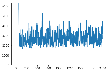
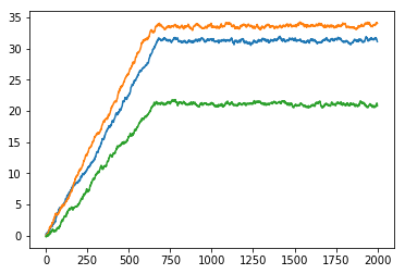
You'll notice in the code that I've added a starting value for $C$ (start_c) and a value for when it has partly converged (warm_c). This code for illustration, as it is a strange assumption that the algorithm is "warm" after 30 iterations.
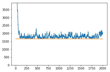
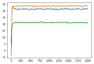
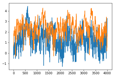
You can see in the plots below what the effect of this is.
$$c_{\text{start}} = 1, c_{\text{warm}} = 1$$
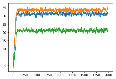
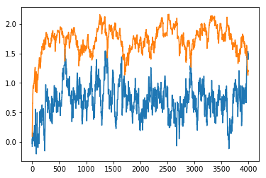
$$c_{\text{start}} = 0.1, c_{\text{warm}} = 0.1$$
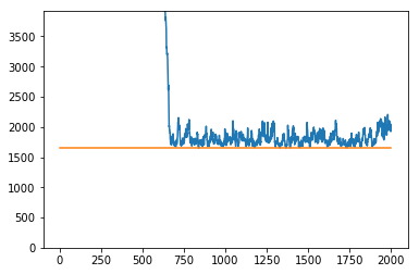
$$c_{\text{start}} = 3, c_{\text{warm}} = 0.1$$
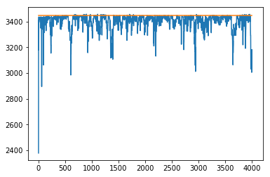
Classification
We can repeat this exercise for classification too.
import numpy as np
import sklearn
from sklearn.datasets import make_classification

X, y = make_classification(n_samples=4000, n_features=2, n_redundant=0,
                           random_state=42, n_clusters_per_class=1)
mod_lmc = sklearn.linear_model.LogisticRegression()
normal_acc = np.sum(mod_lmc.fit(X, y).predict(X) == y)

start_c = <value>
warm_c = <value>

mod_pac = sklearn.linear_model.PassiveAggressiveClassifier(C=start_c)
acc = []
coefs = []
for i, x in enumerate(X):
    mod_pac.partial_fit([x], [y[i]], classes=[0,1])
    coefs.append(mod_pac.coef_.flatten())
    acc.append(np.sum(mod_pac.predict(X) == y))
    if i == 30:
        mod_pac.C = warm_c
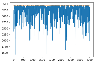
The code is very similar, the only difference is that we are now working on a classification problem.
$$c_{\text{start}} = 1, c_{\text{warm}} = 1$$
$$c_{\text{start}} = 0.1, c_{\text{warm}} = 0.1$$
$$c_{\text{start}} = 0.1, c_{\text{warm}} = 0.1$$
It seems like this $C$ hyperparameter is something to keep an eye on if these sorts of algorithms are within your interest.
Conclusion on Applications
It is nice to see that we're able to have a model work in a streaming setting. I would wonder how often this is useful though, mainly because you need a label to be available in streaming to actually be able to learn from it. One can wonder, if the label is available at streaming then why have the need to predict it?
Then again, all passive agressive linear models have a nice and simple update rule and this can be extended to include matrix factorisation models. For large webshops this is very interesting because it suggests a method where you may be able to update per click. For a nice hint at this, check out this presentation from flink forward.
Conclusions on Elegance
The bayesian inside of me can't help but see an analogy to something bayesian happening here too. We update our prior belief (weights at time $n$) if we see something that we did not expect. By doing this repeatedly we come to a somewhat recusive model that feels very similar to bayesian updating.
$$ p(w_{n+1}| D, d_{n+1}) \propto p(d_{n+1} | w_n) p(w_n)$$
Bayesian updating seems more appealing because we get to learn from every datapoint which also has a regularisation functionality (it removes both the passive and the agressive aspect from the update rule). The main downside will be the datastructure though, which is super easy with this passive aggressive approach.